


Before we begin with A/B testing, it is of the utmost importance that we understand Hypothesis testing first.
In simple words hypothesis is an idea that can be tested, and in hypothesis testing we are trying to reject the STATUS QUO, thereby trying to find an alternative change or innovation
Let us suppose that we are primarily concerned with using the resulting sample to test some particular hypothesis concerning them. As an illustration, suppose that a construction firm has just purchased a large supply of cables that have been guaranteed to have an average of breaking strength of at least 7,000 psi. To verify this claim, the firm decided to take a random sample of 10 of these cables to determine their breaking strengths. They will then use the result of this experiment to ascertain whether or not they accept the cable manufacturer’s hypothesis that the population mean is at least 7,000 pounds per square inch.
Mathematically, a statistical hypothesis is usually a statement about a set of parameters of a population distribution. It is called hypothesis because it is not known whether or not it is true.
A primary problem is to develop a procedure for determining whether or not the values of a random sample from this a population are consistent with the hypothesis. For instance, consider a particular normally distributed population having an unknown mean value of θ and known variance of 1. The statement “θ is less than 1” is a statistical hypothesis that we could try to test by observing a random sample from this population. If the random sample is deemed to be consistent with the hypothesis under consideration, we say that the hypothesis level has been “accepted”; otherwise we say we cannot “accept it”.
In “accepting” a given hypothesis we are not actually claiming it is true but rather we are saying that the resulting data appears to be consistent with it.
Significance levels
Consider a population having distribution Fθ, where θ is unknown, and suppose we want to test a specific hypothesis about θ. We shall denote this hypothesis by Hθ and call it null hypothesis. For example, if Fθ is a normal distribution function with mean θ and variance equal to 1 then two possible null hypotheses about θ are:
a) Hθ : θ=1
b) Hθ : θ≤1
Thus the first of these hypotheses states that the population is normal with mean 1 and variance 1, whereas the second states that it is normal with variance 1 and a mean less than or equal to 1. Note that the null hypothesis in (a), when true, completely specifies the population distribution; whereas the null hypothesis in (b) does not. A hypothesis that, when true, completely specifies the population distribution is called a simple hypothesis and one that doesn’t is called a composite hypothesis.
Level of significance is the degree of significance in which we accept or reject the null-hypothesis. 100% accuracy is not possible for accepting or rejecting a hypothesis, so we therefore select a level of significance that is usually 5%.
This is normally denoted with α and generally it is 0.05 or 5% , which means your output should be 95% confident to give similar kind of result in each sample.
Critical Region
Suppose now that in order to set a specific null hypothesis H0, a population sample of size n — say X1,…Xn — is to be observed. Based on these n values, we must decide whether or not to accept H0. A test for H0 can be specified by defining a region C in n-dimensional space with the proviso that the hypothesis is to be rejected if the random sample X1,…,Xn turns out to lie in C and accepted otherwise. The region C is called the critical region. In other words, the statistical test determined by the critical region.
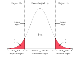
In other words, the statistical test determined by the critical region C is the one that
accepts H0 if (X1,X2,…Xn) ∉ C
rejects H0 if (X1,…,Xn) ∈ C
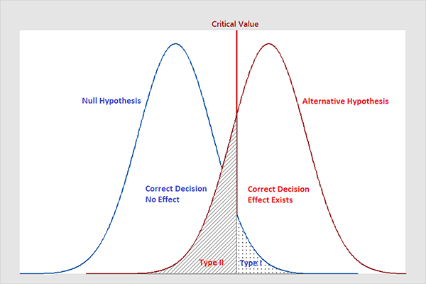
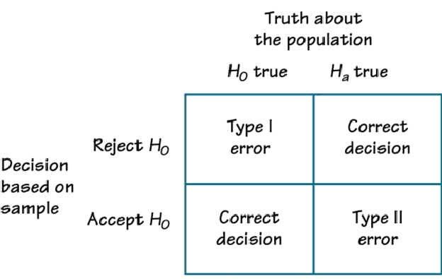
It is important to note when developing a procedure for testing a given null hypothesis H0, that, in any test, two different types of errors can result. The first of these, called a type I error, is said to result if the test incorrectly calls for rejecting H0 when it is indeed correct. The second, called a type II error, results if the test calls for accepting H0 when it is false.
Sounds a little too mathematical, doesn’t it? Let us understand the types of error with a very fun example
Suppose we have a crush on someone and are unsure if we should invite them out on a date. So what are the probabilities of each scenario?

Let us assume the null hypothesis to be H0: They don’t like you (and you don’t ask them out)
The truth can be put in 4 scenarios:
- They don’t like you and you don’t ask them out ←Correct decision
- They like you and you don’t ask them out(missed chance)/False negative← Type II error
- They don’t like you and you ask them out / False positive ← Type I error
- They like you and you ask them out ← Correct decision
Only if Mathematics could solve the matters of love!
P Value
The P value, or calculated probability, is the probability of finding the observed, or more extreme, results when the null hypothesis (H 0) of a study question is true — the definition of ‘extreme’ depends on how the hypothesis is being tested.
If your P value is less than the chosen significance level then you reject the null hypothesis i.e. accept that your sample gives reasonable evidence to support the alternative hypothesis. It does NOT imply a “meaningful” or “important” difference; that is for you to decide when considering the real-world relevance of your result.
Example : you have a coin and you don’t know whether that is fair or tricky so let’s decide null and alternate hypothesis
H0 : a coin is a fair coin.
H1 : a coin is a tricky coin. and alpha = 5% or 0.05
Now let’s toss the coin and calculate p- value ( probability value).
Toss a coin 1st time and result is tail- P-value = 50% (as head and tail have equal probability)
Toss a coin 2nd time and result is tail, now p-value = 50/2 = 25%
and similarly we Toss 6 consecutive time and got result as P-value = 1.5% but we set our significance level as 95% means 5% error rate we allow and here we see we are beyond that level i.e. our null- hypothesis does not hold good so we need to reject and propose that this coin is a tricky coin which is actually.
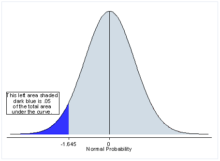
One tailed and Two tailed tests
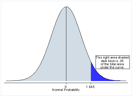
One Tailed Test: A test of a statistical hypothesis , where the region of rejection is on only one side of the sampling distribution , is called a one-tailed test.
For ex: Let us compare the mean of a sample to a given value x using a t-test. Our null hypothesis is that the mean is equal to x. A one-tailed test will test either if the mean is significantly greater than x or if the mean is significantly less than x, but not both. Then, depending on the chosen tail, the mean is significantly greater than or less than x if the test statistic is in the top 5% of its probability distribution or bottom 5% of its probability distribution, resulting in a p-value less than 0.05.
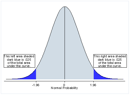
Two Tailed Test: A two-tailed test is a statistical test in which the critical area of a distribution is two-sided and tests whether a sample is greater than or less than a certain range of values. If the sample being tested falls into either of the critical areas, the alternative hypothesis is accepted instead of the null hypothesis.
For ex: We wish to compare the mean of a sample to a given value x using a t-test. Our null hypothesis is that the mean is equal to x. A two-tailed test will test both if the mean is significantly greater than x and if the mean significantly less than x. The mean is considered significantly different from x if the test statistic is in the top 2.5% or bottom 2.5% of its probability distribution, resulting in a p-value less than 0.05.
Popular Hypothesis Testing Methods:
- When Variance is known: Z-Test:
We use Z- test when the following conditions are true:
Sample size is greater than 30
Population data is normally distributed, this doesn’t matter if the first condition is true
Exclusion/Inclusion of one data point is independent of inclusion/exclusion of another data point
Sample is randomly selected
All Sample sizes are equal
One-sample Z-Test:

Two-sample Z-Test:

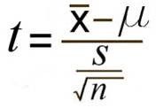
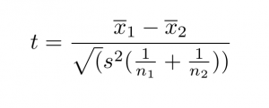
- When Variance is not known: T-Test:
T-tests are conducted when the following conditions are true:
Population variance is unknown
Sample size is less than 30
One-sample T-Test:
Two-sample T-test:
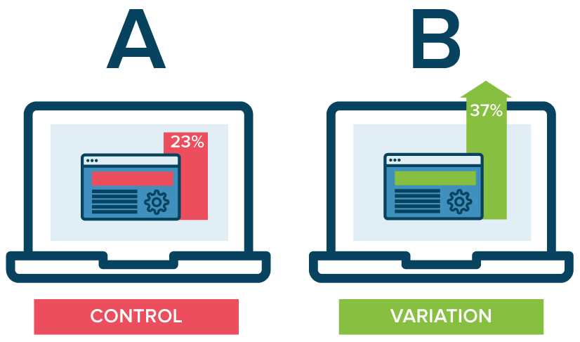
A/B Testing:
So What is A/B Testing?
A/B testing is a method of statistical hypothesis testing wherein two variants of a web page are compared against one another to understand which one performs better for a conversion goal.
Why do A/B testing?
We do A/B testing because cannot have a 100% accuracy of how the next 100,000 people who visit the web page will behave. We cannot wait until that happens for optimizing the experience because it will be too late by then.
Therefore we use the information we have now to make predictions of future behavior by statistical analysis. Or in simple words, keep a track on the 1,000 customer behavior to estimate the behavior of the next 99,000 users.
If we can optimize our statistical analysis will incredible efficiency, this will prove extremely beneficial for running the business.
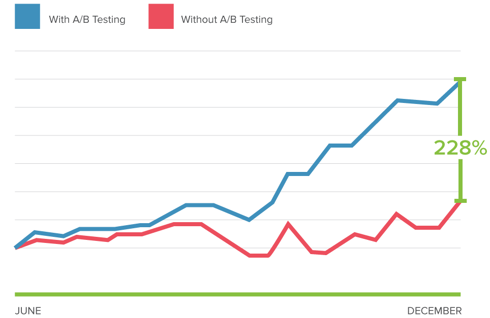
Let us look at an example of sales before and after A/B testing
Where should we be careful?
Since we are trying to make predictions about the population, our sample needs to accurately represent the population.
Let us look at a split testing dashboard to understand Confidence level and margin of error:
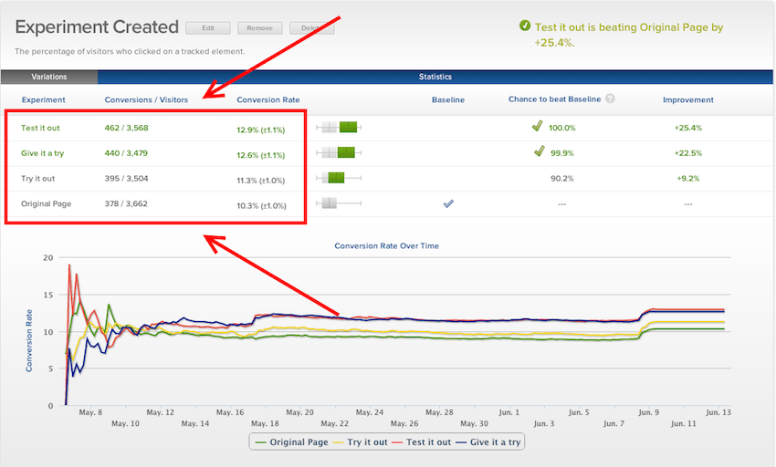
The original page has a conversion rate of 10.3% plus/minus 1%. The 10.3% is the true mean. This 1% is our margin of error. Although we want to have 100% confidence of true mean. In real life scenarios that would inaccurate.
Hence 10.3% ± 1.0 % at 95% confidence is our actual conversion rate for this page
So, what we are saying is that if 20 samples were taken, we can say with complete certainty that 19 0f those would contain true conversion rate within 95% confidence intervals.
The confidence interval is an observed range in which a given percentage of test outcomes fall. We manually select our desired confidence level at the beginning of our test, and the size of the sample we need is based on our desired confidence level.
The range of our confidence level is then calculated using the mean and the margin of error.
The upper bound of the confidence interval is found by adding the margin of error to the mean. The lower bound is found by subtracting the margin of error from the mean.
Errors:
As we already mentioned, A/B testing will not be done for the entire population but a small sample for example lets say 1,000 people and make a hypothesis that Variation B will perform better than Variation A.
If Variation A has better conversion then no change needs to be made since this is our original page.
If Variation B performs better then we have to determine if the change was statistically large enough for it to effect the population and if yes then we must make changes according to Variation B.
So why can’t we directly do this? Because of the variance of samples. There can be 4 scenarios that occur when we run our test.
- Test says Variation B is better and Variation B is actually better.
- Test says Variation B is better but Variation B is not better- ←Type I error
- Test says Variation B is not better but Variation B is better ← Type II error
- Test says Variation B is not better and Variation B is actually not better
Type I Errors & Statistical Significance
A type I error occurs when we incorrectly reject the null hypothesis.
To put this in AB testing terms, a type I error would occur if we concluded that Variation B was “better” than Variation A when it actually was not.
Remember that by “better”, we aren’t talking about the sample. The point of testing our samples is to predict how a new page variation will perform with the overall population. Variation B may have a higher conversion rate than Variation A within our sample, but we don’t truly care about the sample results. We care about whether or not those results allow us to predict overall population behavior with a reasonable level of accuracy.
Type I error is related to Statistical Significance.
Type II Errors & Statistical Power
A type II error occurs when the null hypothesis is false, but we incorrectly fail to reject it.
To put this in AB testing terms, a type II error would occur if we concluded that Variation B was not “better” than Variation A when it actually was better.
Just as type I errors are related to statistical significance, type II errors are related to statistical power, which is the probability that a test correctly rejects the null hypothesis.
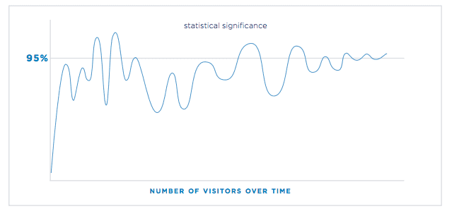
AB tester are mostly interested in Statistical Significance, but over a course of test the values will go from significant to non significant. Hence it is important to have a large enough sample space over a consistent time period to account for the variability of population.
It is important to take the sample size and time pre-decided in advance. Do not use Statistical significance as a stopping factor because the test results will oscillate between significant and not significant. The only time you should use significance as the deciding factor is at the endpoint.
A/B Testing Examples: