

Data Science
The Bayes' Theorem Made Simple
Last Updated: 12th October, 2023

Narender Ravulakollu
Technical Content Writer at almaBetter
Have you ever wondered how doctors come up with a diagnosis? Or how insurance companies calculate your interest rate? Or how detectives solve a crime? All of these people use a method called the Bayes’ Theorem.

Bayes’ Theorem is a way to calculate the probability of something happening, given that something else has already happened. It is used in many different fields, ranging from medicine to criminology.
For example, let’s say you are trying to figure out the probability that it will rain tomorrow. You might start by looking at the weather forecast, which might give you a 60% chance of rain.
Then you remember that the weather forecast is often wrong. In fact, historical data shows that the weather forecast is only right about 80% of the time.
So, using Bayes’ Theorem, you can combine the 60% chance of rain from the forecast with the 80% chance that the forecast is right, to get a more accurate estimate of the probability of rain tomorrow.
Here’s how it works in a layperson’s words:
Let’s consider Charan, Suresh, Mahesh, and Rohan were four people in your hostel. When you were working late at night, you saw someone in the kitchen, and you didn’t notice who he was.
Let’s calculate the probabilities, P(Charan) = 0.25, P(Suresh) = 0.25, P(Mahesh) = 0.25, and P(Rohan) = 0.25.
Now we will give you some extra information, The person had a blue hoodie. Charan wears a blue hoodie 2 times a week. Suresh wears a blue hoodie 3 times a week. Mahesh wears a blue hoodie once a week. Rohan wears a blue hoodie 4 times a week.
Let us now compute the probabilities using this new information. Probability that Charan was in the kitchen is 2/10 i.e, P(Charan) = 0.2 Probability that Suresh was in the kitchen is 3/10 i.e, P(Suresh) = 0.3 Probability that Mahesh was in the kitchen is 1/10 i.e, P(Mahesh) = 0.1 Probability that Rohan was in the kitchen is 4/10 i.e, P(Rohan) = 0.4 Prior probabilities are those calculated before the new information, while posterior probabilities are those calculated after the new information.
Let’s dive into a more detailed explanation
Consider a scenario where Charan stays in the hostel for 3 days a week, Suresh stays in the hostel for 4 days a week, Mahesh stays in the hostel for 5 days a week, and Rohan stays in the hostel for 6 days a week.
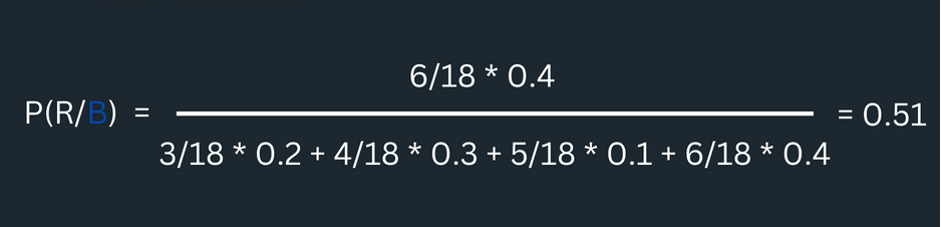
Let’s calculate the probabilities, Probability that Charan was in the kitchen is 3/18 i.e, P(Charan) = 3/18 Probability that Suresh was in the kitchen is 4/18 i.e, P(Suresh) = 4/18 Probability that Mahesh was in the kitchen is 5/18 i.e, P(Mahesh) = 5/18 Probability that Rohan was in the kitchen is 6/18 i.e, P(Rohan) = 6/18
Let’s look at the below image for better understanding:
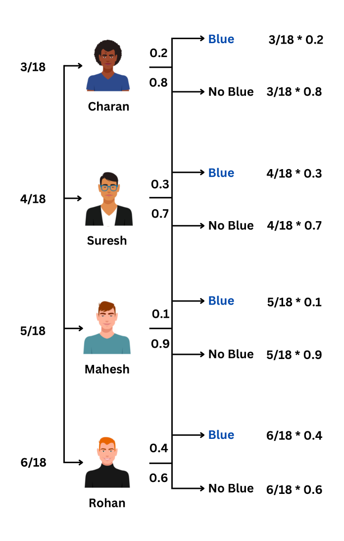
Probability that the person is Charan is 3/18, Suresh is 4/18, Mahesh is 5/18 and Rohan is 6/18. These are the four cases. Probability that Charan wears a blue hoodie is 0.2 and probability that Charan does not wear a blue hoodie is 0.8. In the case of Suresh, probability that Suresh wears a blue hoodie is 0.3 and probability that Suresh does not wear a blue hoodie is 0.7.
Probability that Mahesh wears a blue hoodie is 0.1 and probability that Mahesh does not wear a blue hoodie is 0.9. In the case of Rohan, the probability that Rohan wears a blue hoodie is 0.4 and probability that Rohan does not wear a blue hoodie is 0.6.
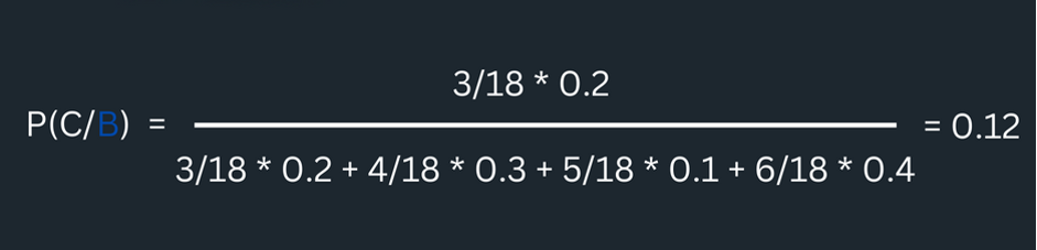
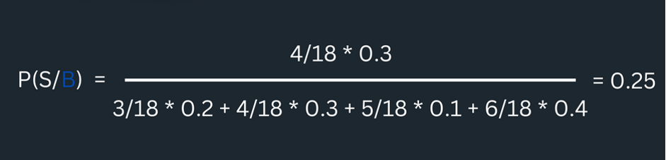
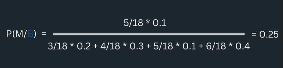
Since we are only interested in events that have blue hoodies, we ignore other events. Normalize the probabilities we get
Probability that the person wearing a blue hoodie is Charan is:
Probability that the person wearing a blue hoodie is Suresh is:
Probability that the person wearing a blue hoodie is Mahesh is:
Probability that the person wearing a blue hoodie is Rohan is:
We have successfully crossed the bridge.
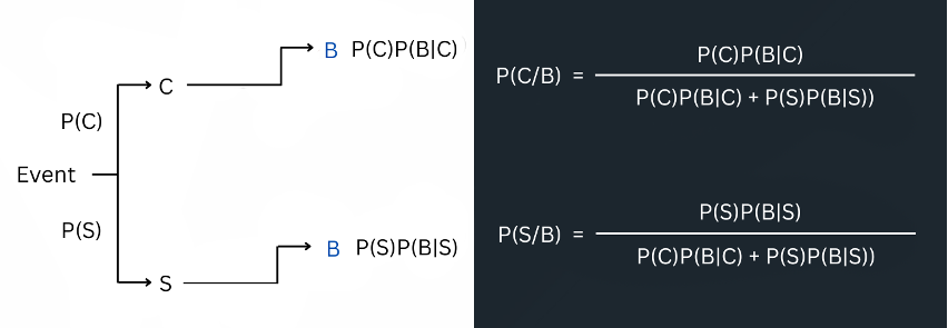
Deriving the Formulae
We can derive the following formulae from what we have learnt above:
Conclusion: Bayes’ Theorem is a powerful statistical tool that can be used to calculate the probability of an event occurring, given that another event has already occurred. This theorem can be applied to a variety of situations, from medical diagnosis to stock market prediction.
By using Bayes’ Theorem, we can better understand the relationships between different events and make more informed decisions.
If you are a diligent Data Science enthusiast and are eager to enter the industry, we have the perfect opportunity for you. Sign up for our upcoming Full Stack Data Science batch to kickstart your career, today!
Read our latest blog on “5 real-time use cases of ANOVA”.
Related Articles
Top Tutorials

Made with in Bengaluru, India


- Join AlmaBetter
- Sign Up
- Become A Coach
- Coach Login
- Policies
- Privacy Statement
- Terms of Use
- Contact Us
- admissions@almabetter.com
- 08046008400
- Official Address
- 4th floor, 133/2, Janardhan Towers, Residency Road, Bengaluru, Karnataka, 560025
- Communication Address
- Follow Us

© 2025 AlmaBetter