Data Preprocessing in Machine Learning

Lets understand the various types data preprocessing in machine learning and data preprocessing techniques. The data cleaning in data preprocessing prepares the available data for further machine learning process to reach the client’s requirement.

What is a Data?

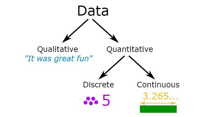
Data is a collection of facts, such as numbers, words, measurements, observations, or just descriptions of things.

A Data Visualization

There are mainly three types of data that you will encounter while doing Data Science. Those are Numerical & Categorical, Textual, and Image Data. Let’s deep dive into the Data Pre-processing factory and let’s know what’s actually happening in the factory.

What is Data Preprocessing in Machine Learning?

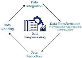
Data Preprocessing in Data Mining

Data preprocessing in machine learning is a process of preparing the raw data and making it suitable for a machine learning model. It is the first and crucial step while creating a machine learning model. It is a data mining technique that involves the transformation of raw data into an insightful and organized format. A real-world data generally contains noises, missing values, and maybe in an unusable format that cannot be directly used for machine learning models. For resolving such issues it prepares raw data for further processing. Data preprocessing is a required task for cleaning the data and making it suitable for a machine learning model which also increases the accuracy and efficiency of a machine learning model.

Why Do We Need Data Preprocessing?

Data preprocessing is an integral step in Machine Learning as the quality of data and the useful information that can be derived from it directly affects the ability of our model to learn; therefore, we must preprocess our data before feeding it into our model. Real-world data is often incomplete, inconsistent, lacking in certain behaviors or trends, and is likely to contain many errors. To better visualize and extract the hidden pattern, Data Preprocessing must be done.

What are Features of Data Preprocessing?

Now the world is full of data. There are billions of data created every day and they are getting stored in databases through a proper channel as well as a proper order. Those are called datasets. A Dataset is nothing but a collection of samples or observations organized with some columns and separated from each other. Those columns that tell the properties and qualities of any object or final output are known as independent columns or features. The Dependent columns are the final output of the features. In other words, features are the traits of the dataset otherwise called Variable and Attribute. For example, RAM, storage, and model could be considered as features of a Smart Phone. However these could belong to different data types, and we might have to deal with them differently.

Various Types of Data in Data Preprocessing

Now we will deep dive into some data preprocessing techniques for various data types.

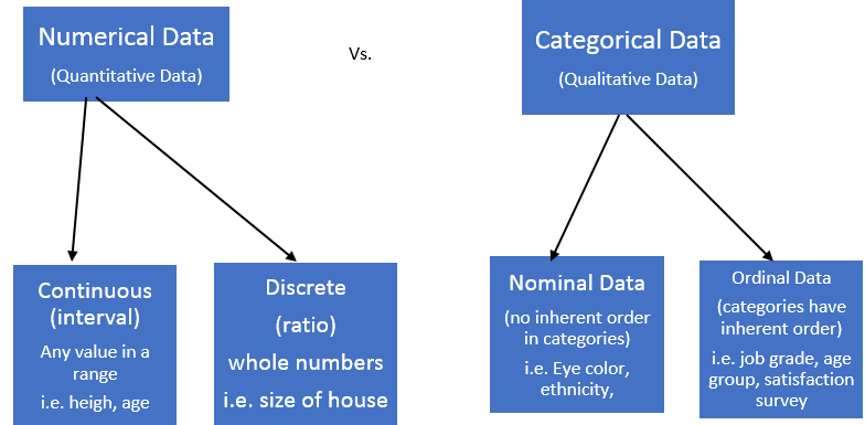
Numerical & Categorical Data

Numerical data is a data type expressed in numbers, rather than natural language description. Sometimes called quantitative data, numerical data is always collected in number form. Categorical variables represent types of data that may be divided into groups. Examples of categorical variables are race, sex, age group, and educational level.

Data Preprocessing Steps and Techniques

Feature Engineering

Feature engineering is the process of transforming raw data into features that better represent the underlying problem to the predictive models, resulting in improved model accuracy on unseen data.

Handling Missing Values

Handling the missing values is one of the greatest challenges faced by analysts because making the right decision on how to handle it generates robust data models. Let us look at different ways of imputing the missing values.

Mean/Median/Mode Replacement

Mean/Median/Mode imputation has the assumption that the data are missing completely at Random. We solve this by replacing the NaN value with the most frequent occurrence of the variables. In the case of the categorical variables, we can use mode.

Random Sample Imputation

Random Sample imputation consists of taking random observation from the dataset and we use this observation to replace the NaN variable. It assumes the data are missing completely at random.

Capturing NaN value with a new feature

It works well if the data are not missing completely at random. Let there is a feature named Age, and some of the values are missed. Thus, we can create another feature while replacing NaN with 1 and non-NaN with 0.

End of Distribution Imputation

Here, we will find out the extreme value of the distribution and impute that in the place of missing values. It’s easy to implement and captures the importance of missingness if there is one.

Arbitrary Imputation

This technique was derived from the Kaggle competition as it consists of replacing NaN with an arbitrary value.

Frequent Categories Imputation

It is used where a very less number of missing values are present. It’s otherwise known as the mode imputation while the total count of the mode value will be imputed. It’s easy and fast to implement.

Creating a Sub-model to predict the missing value.

Here, we will create a sub-model while taking the non-missing value as a separate dataset(we will split and create a model with this dataset) and the missing vale as another dataset whose values are to be predicted.

Deleting Column if missing value > 60%

If the complete row is having NaN values then it doesn’t make any value out of it. So such rows/columns are to be dropped immediately. Or if the % of row/column is mostly missing say about more than 60% then also one can choose to drop.

Using Algorithms Which Support Missing Values

KNN is a machine learning algorithm that works on the principle of distance measure. This algorithm can be used when there are nulls present in the dataset. While the algorithm is applied, KNN considers the missing values by taking the majority of the K nearest values. In this particular dataset, taking into account the person’s age, sex, class, etc, we will assume that people having the same data for the above-mentioned features will have the same kind of fare.

Unfortunately, the SciKit Learn library for the K — Nearest Neighbour algorithm in Python does not support the presence of the missing values.

Another algorithm that can be used here is RandomForest. This model produces a robust result because it works well on non-linear and categorical data. It adapts to the data structure taking into consideration of the high variance or the bias, producing better results on large datasets.

Checking for duplicates

If the same row or column is repeated, you can also drop it by keeping the first instance. So that while running machine learning algorithms, so as not to offer that particular data object an advantage or bias.

Handling Outliers

An outlier is an observation that lies an abnormal distance from other values in a random sample from a population. In a sense, this definition leaves it up to the analyst (or a consensus process) to decide what will be considered abnormal. Before abnormal observations can be singled out, it is necessary to characterize normal observations. A point beyond an inner fence on either side is considered a mild outlier. A point beyond an outer fence is considered an extreme outlier.

Handling Outliers is a good practice before passing the data to the ML model as we can get a better model with good metrics.

Using Standard Deviation in Symmetric Curve

In a Gaussian distribution while it’s the symmetric curve and outlier are present. Then, we can set the boundary by taking standard deviation into action.

Using IQR in skew-symmetric Curve

The box plot is a useful graphical display for describing the behavior of the data in the middle as well as at the ends of the distributions. The box plot uses the median and the lower and upper quartiles (defined as the 25th and 75th percentiles). If the lower quartile is Q1 and the upper quartile is Q3, then the difference (Q3 — Q1) is called the interquartile range or IQ. A box plot is constructed by drawing a box between the upper and lower quartiles with a solid line drawn across the box to locate the median. The following quantities (called fences) are needed for identifying extreme values in the tails of the distribution:

• lower inner fence: Q1–1.5*IQ
• upper inner fence: Q3 + 1.5*IQ
• lower outer fence: Q1–3*IQ
• upper outer fence: Q3 + 3*IQ

Using Outlier Insensitive Algorithms

Some algorithms that are not sensitive to outliers are Naive Bayes Classifier, Support Vector Machine, Decision Tree, Ensemble Techniques, and K-Nearest Neighbours. We can use these algorithms to get rid of outliers.

Categorical Encoding

This means that categorical data must be encoded into numbers before we can use it to fit and evaluate a model. There are many ways to encode categorical variables for modeling as follows.

Nominal Encoding

Variable comprises a finite set of discrete values with no relationship between values. Some examples include:

A “pet” variable with the values: “dog” and “cat“. A “color” variable with the values: “red“, “green“, and “blue“. A “place” variable with the values: “first“, “second“, and “third“

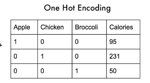
One Hot Encoding

One Hot Encoding means to encode or create additional features for all unique categorical values. For example, ‘Apple’, ‘ Chicken’, and ’Brocoli’ have been encoded as 1 in that place only where it is present.

• One Hot Encoding with many categorical

It is the same as one-hot encoding but the difference is Let you have more than 20 unique categories. Then if you will perform one-hot encoding to all those you will have additional 20 columns. This will lead to the Curse of Dimensionality. So, It has been observed from the KDD Orange Cup challenge that some top n no. of maximum categories are taken and encoded.

• Mean Encoding

Here, You will calculate the mean of the unique categories to the no. of occurrence in that dataset and encode them while creating a new column.

• Ordinal Encoding

Variable comprises a finite set of discrete values with a ranked ordering between values. In ordinal encoding, each unique category value is assigned an integer value. For example, “red” is 1, “green” is 2, and “blue” is 3.

• Label Encoding

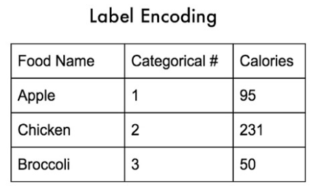
In this type of encoding, You have to encode the unique categories as per their rating as shown in the above image.

• Target guided Ordinal Encoding

First, you have to calculate the mean as same in mean encoding but here you won’t encode them with their mean values. Here, you will have to perform label encoding based on those mean values. so, in other words, “target guided ordinal encoding = mean encoding +label encoding.”

• Count (or) Frequency Encoding

In this type of encoding, you have to encode the unique categories by their total no. of occurrences in that dataset and particularly in that categorical column.

• Probability ratio Encoding

This encoding is purely based on probability. If it’s possible to calculate the probability or it’s a probability type problem, You can use this type of encoding by calculating the probabilities. For example, If you are working with some dataset like survive and not- survive in “Titanic Dataset”. There you can use probability encoding.

Data Transformation

It refers to putting the values in the same range or same scale so that no variable is dominated by the other. Most of the time, the collected data set contains features highly varying in magnitudes, units, and ranges. If scaling is not done then the algorithm only takes magnitude into account and not units hence incorrect modeling. To solve this issue, we have to do scaling to bring all the variables to the same level of magnitude.

Standardization

Standardization is another scaling technique where the values are centered around the mean with a unit standard deviation. This means that the mean of the attribute becomes zero and the resultant distribution has a unit standard deviation.

Normalization

Normalization is a scaling technique in which values are shifted and rescaled so that they end up ranging between 0 and 1. It is also known as Min-Max scaling.

Robust Scaler

It is used to scale the feature to median and quantile. Scaling using median and quantiles consists of subtracting the median from all the observations and then dividing by the interquartile difference. The inter quantile difference is the difference between the 75th and 25th.

Gaussian Transformation

Some machine learning algorithms like linear and logistic regression assume that the features are normally distributed. So, we need to transform the features by the following methods. Logarithmic Transformation: Transforming using a logarithmic function. (ex: np.log(df[‘’]))

Inverse Transformation: Transforming using an inverse function. (ex: 1/(df[‘’]))

Square Root Transformation: Transforming using a square function. (ex: np.sqrt(df[‘’])

Exponential Transformation: Transforming using an exponential function. (ex: (df[‘’])**(1/1.2))

Box-Cox Transformation: A Box-Cox transformation is a transformation of a non-normal dependent variable into a normal shape. Normality is an important assumption for many statistical techniques; if your data isn’t normal, applying a Box-Cox means that you can run a broader number of tests.

The Box-Cox transformation is named after statisticians George Box and Sir David Roxbee Cox who collaborated on a 1964 paper and developed the technique.

T(y)=(y exp(lambda)-1)/(lambda)

where y is the response variable and ‘lambda’ is the transformation parameter from -5 to 5. In the transformation, all values of ‘lambda’ are considered and the optimal value for a given variable is selected.

Noisy Data

Noisy data is just meaningless. This type of data has no interpretation for machines. There are several reasons behind this i.e., poor and faulty data collection, data entry errors, and so on. It can be handled in the following ways:

Binning Method

To use this method we have to sort the data first. Because this method works on sorted data to smooth it. we have to divide the whole data into two segments of equal size, and no. of methods will be performed to complete the task. here, we consider each segment as a separate one and can be replaced by its boundary values or mean to complete the task.

Clustering

This approach involves the similar feature data groups to be a cluster. If any outliers present, they might be undetected or don’t fall inside the clusters.

For example, We have lots of student data and we want to perform work on those having AI knowledge. Thus we will cluster only those students who know AI.

Regression

We have to assume a regression function before this method. Here data can be made smooth by fitting the data into that function. The regression function we have to assume might be linear one (having one independent variable) or multiple (having multiple independent variables).

Handling Imbalanced Dataset

Dealing with imbalanced datasets entails strategies such as improving classification algorithms or balancing classes in the training data (data preprocessing) before providing the data as input to the machine learning algorithm. The latter technique is preferred as it has wider application.

The main objective of balancing classes is to either increase the frequency of the minority class or decrease the majority class’s frequency. This is done to obtain approximately the same number of instances for both classes. Let us look at a few resampling techniques:

Cross-Validation

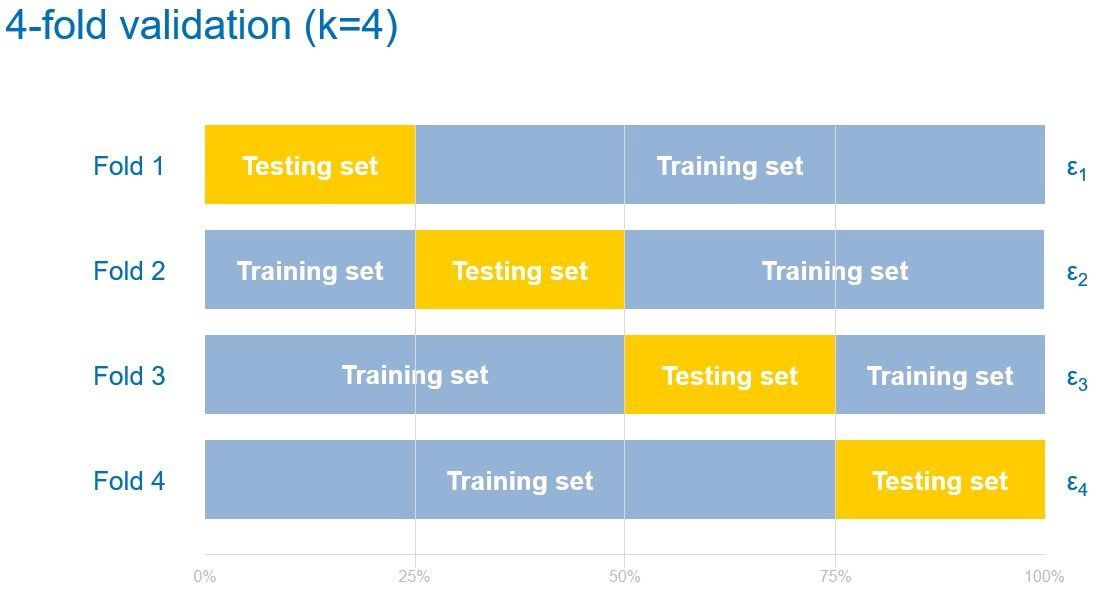
Cross-validation is a resampling procedure used to evaluate machine learning models on a limited data sample. The procedure has a single parameter called k that refers to the number of groups that a given data sample is to be split into. As such, the procedure is often called k-fold cross-validation.

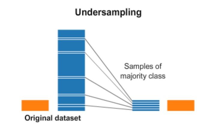
Under Sampling

Undersampling can be defined as removing some observations of the majority class. This is done until the majority and minority class is balanced out.

Undersampling can be a good choice when you have a ton of data -think millions of rows. But a drawback to undersampling is that we are removing information that may be valuable.

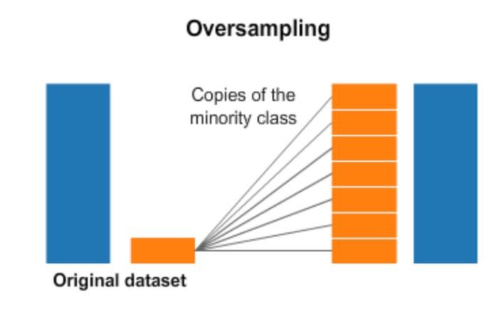
Over Sampling

Oversampling can be defined as adding more copies to the minority class. Oversampling can be a good choice when you don’t have a ton of data to work with.

When undersampling, a con to consider is that it can cause overfitting and poor generalization to your test set.

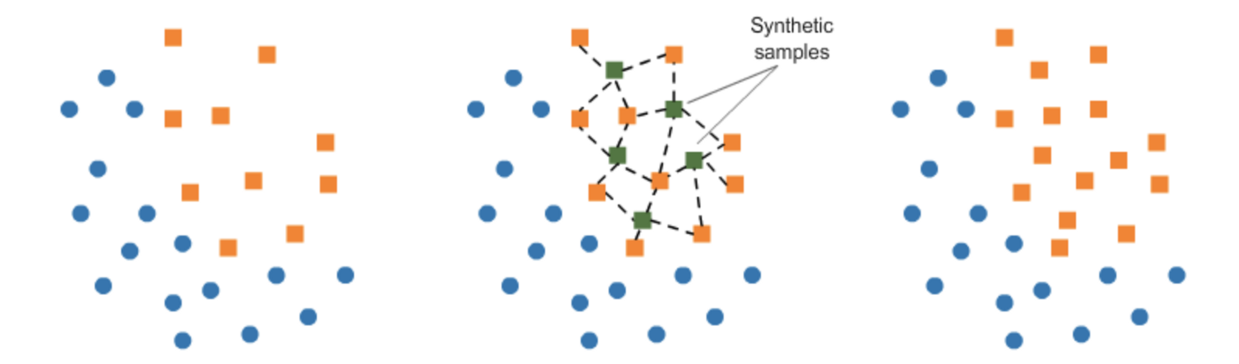
Synthetic Minority over Sampling Technique (SMOTE)

This technique generates synthetic data for the minority class. SMOTE (Synthetic Minority Oversampling Technique) works by randomly picking a point from the minority class and computing the k-nearest neighbors for this point. The synthetic points are added between the chosen point and its neighbors.

Tree-Based Algorithm

While in every machine learning problem, it’s a good rule of thumb to try a variety of algorithms, it can be especially beneficial with imbalanced datasets.

Decision trees frequently perform well on imbalanced data. In modern machine learning, tree ensembles (Random Forests, Gradient Boosted Trees, etc.) almost always outperform singular decision trees, so we’ll jump right into those: Tree base algorithm work by learning a hierarchy of if/else questions. This can force both classes to be addressed.

Data Integration

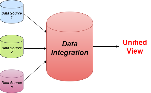
Data Integration is nothing but a data preprocessing technique that combines data from multiple sources while providing users a unified view of these data. For example, In a school, the school authority wants to conduct an interschool competition between three schools. Now school 1 has its own student data but it will collect other school’s student data from different sources and add them up which is called data integration and the outcome data will be a unified view. The condition for data integration is they must have the same entity and similar features. There are mainly 2 major approaches for data integration:-

Tight Coupling

In tight coupling, data is combined from different sources into a single physical location through the process of ETL — Extraction, Transformation, and Loading.

Loose Coupling

In loose coupling data only remains in the actual source databases. In this approach, an interface is provided that takes a query from the user and transforms it in a way the source database can understand, and then sends the query directly to the source databases to obtain the result.

Data Reduction

data reduction picture representation

Let us assume we have a dataset of billions of rows of data. Now we will require high computationally cost and timing cost to work on that population. So, Here Data reduction comes in handy. Data reduction is a process that reduced the volume of original data and represents it in a much smaller volume. Data reduction techniques ensure the integrity of data while reducing the data. It is done to avoid the curse of dimensionality. Curse of Dimensionality refers to a set of problems that arise when working with high-dimensional data and working with high dimensionality we will have a chance of overfitting. So, without changing the feature and deleting the attributes

Dimensionality Reduction

Dimensionality reduction eliminates the attributes from the data set under consideration thereby reducing the volume of original data. In the section below, we will discuss three methods of dimensionality reduction. Those are Wavelet Transform, Principal Component Analysis, and Attribute Subset Selection. It will reduce the data from high dimensionality to low dimensionality.

Numerosity Reduction

The numerosity reduction reduces the volume of the original data and represents it in a much smaller form. This technique includes two types parametric and non-parametric numerosity reduction. Parametric numerosity reduction incorporates ‘storing only data parameters instead of the original data. One method of parametric numerosity reduction is the ‘regression and log-linear method. Non-parametric numerosity reduction involves Histogram, Sampling Techniques, and Data cube aggregation. Sampling Techniques involve several techniques like Random Sampling, Stratified sampling, Selective sampling, and Cluster sampling.

Textual Data

Preprocessing the text data is a very important step while dealing with text data because the text at the end is to be converted into features to feed into the model. The objective of preprocessing text data is that we won’t get rid of characters, words, others that don’t give value to us. We want to get rid of punctuations, stop words, URLs, HTML codes, spelling corrections, etc. We would also like to do Stemming and Lemmatization so that in features duplication of words is not there which convey almost the same meaning.

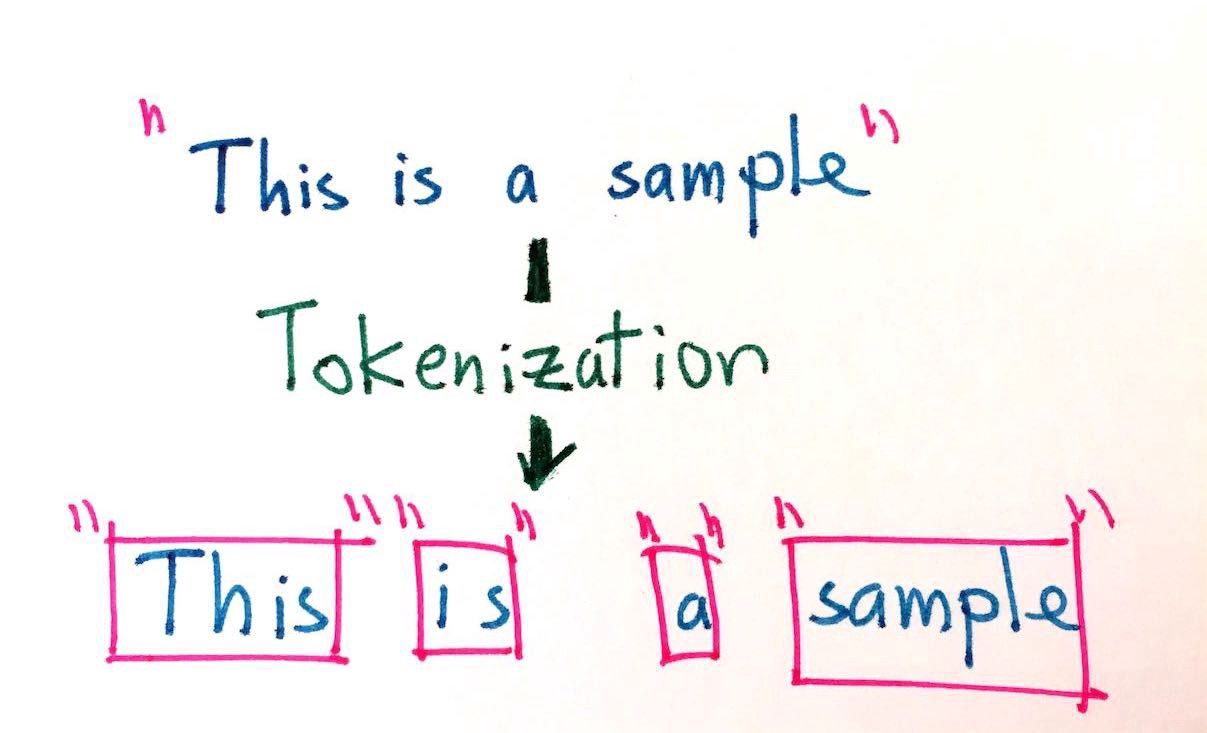
Tokenization

Tokenization is the process of breaking down a piece of text into small units called tokens. A token may be a word, part of a word, or just characters like punctuation. In other words, Tokenization is breaking a text chunk into smaller parts. Whether it is breaking Paragraphs in sentences, sentence into words, or word in characters.

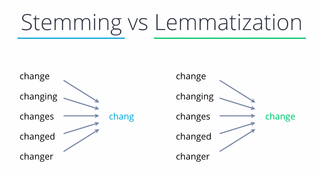
Stemming

Stemming is the process of producing morphological variants of a root/base word. Stemming programs are commonly referred to as stemming algorithms or stemmers. A stemming algorithm reduces the words “chocolates”, “chocolatey”, “choco” to the root word, “chocolate” and “retrieval”, “retrieved”, “retrieves” reduce to the stem “retrieve”. Stemming is an important part of the pipelining process in Natural language processing. The input to the stemmer is tokenized words.

• Porter Stemming

It is one of the most popular stemming methods proposed in 1980. It is based on the idea that the suffixes in the English language are made up of a combination of smaller and simpler suffixes. This stemmer is known for its speed and simplicity. The main applications of Porter Stemmer include data mining and Information retrieval. However, its applications are only limited to English words. Also, the group of stems is mapped onto the same stem and the output stem is not necessarily a meaningful word. The algorithms are fairly lengthy in nature and are known to be the oldest stemmer.

Example: EED -> EE means “if the word has at least one vowel and consonant plus EED ending, change the ending to EE” as ‘agreed’ becomes ‘agree’.

• Snowball Stemming

When compared to the Porter Stemmer, the Snowball Stemmer can map non-English words too. Since it supports other languages the Snowball Stemmers can be called a multi-lingual stemmer. The Snowball stemmers are also imported from the nltk package. This stemmer is based on a programming language called ‘Snowball’ that processes small strings and is the most widely used stemmer. The Snowball stemmer is way more aggressive than Porter Stemmer and is also referred to as Porter2 Stemmer. Because of the improvements added when compared to the Porter Stemmer, the Snowball stemmer is having greater computational speed.

• N-gram Stemming

An n-gram is a set of n consecutive characters extracted from a word in which similar words will have a high proportion of n-grams in common.

Example: ‘INTRODUCTIONS’ for n=2 becomes : I, IN, NT, TR, RO, OD, DU, UC, CT, TI, IO, ON, NS, S

Lemmatization

Lemmatization technique is like stemming. The output we will get after lemmatization is called ‘lemma’, which is a root word rather than root stem, the output of stemming. After lemmatization, we will be getting a valid word that means the same thing. In simpler forms, a method that switches any kind of a word to its base root mode is called Lemmatization.

In other words, Lemmatization is a method responsible for grouping different inflected forms of words into the root form, having the same meaning. It is similar to stemming, in turn, it gives the stripped word that has some dictionary meaning. The Morphological analysis would require the extraction of the correct lemma of each word.

For example, Lemmatization clearly identifies the base form of ‘troubled’ to ‘trouble’’ denoting some meaning whereas, Stemming will cut out the ‘ed’ part and convert it into ‘trouble which has the wrong meaning and spelling errors.

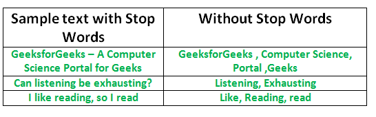
Removing Stop Words

A stop word is a commonly used word (such as “the”, “a”, “an”, “in”) that a search engine has been programmed to ignore, both when indexing entries for searching and when retrieving them as the result of a search query.

We would not want these words to take up space in our database, or taking up the valuable processing time. For this, we can remove them easily, by storing a list of words that you consider to stop words. NLTK(Natural Language Toolkit) in python has a list of stopwords stored in 16 different languages. You can find them in the nltk_data directory.

Vectorizer

Vectorization is the process of converting words into numbers is called Vectorization, Which is a methodology in NLP to map words or phrases from vocabulary to a corresponding vector of real numbers which is used to find word predictions, similarities, etc. The vectorization is used in a use case like Text classification, Compute Similar words, Document Clustering / Grouping, Natural language Processing (NLP), feature extraction in Text Classification.

To vectorize a corpus with a bag-of-words (BOW) approach, we represent every document from the corpus as a vector whose length is equal to the vocabulary of the corpus.

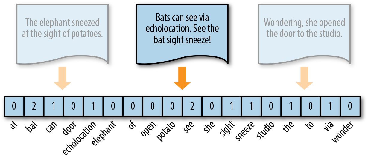
We usually use Count Vectorizer, TF-IDF vectorizer, and Hash vectorizer. Word2vec is a method to efficiently create word embeddings

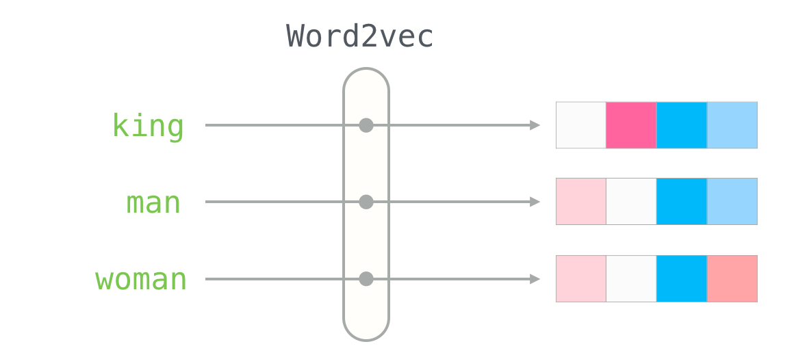
Image Data

Image pre-processing is the term for operations on images at the lowest level of abstraction. These operations do not increase image information content but they decrease it if entropy is an information measure. The aim of pre-processing is an improvement of the image data that suppresses undesired distortions or enhances some image features relevant for further processing and analysis tasks.

• Pixel brightness transformations/ Brightness corrections

Brightness transformations modify pixel brightness and the transformation depends on the properties of a pixel itself. In PBT, the output pixel’s value depends only on the corresponding input pixel value. Examples of such operators include brightness and contrast adjustments as well as color correction and transformations.

Contrast enhancement is an important area in image processing for both human and computer vision. It is widely used for medical image processing and as a pre-processing step in speech recognition, texture synthesis, and many other images/video processing applications.

g(x)=αf(x)+β, alpha and beta control contrast and brightness of the image.

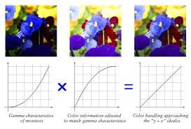
• Gamma correction — You can perform a non-linear adjustment to individual pixel values. While performing image normalization we just do linear operations on individual pixels, i.e. scalar multiplication and addition/subtraction.

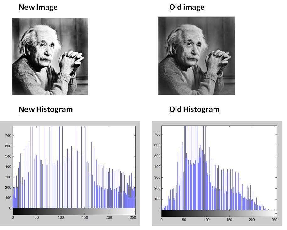
• Histogram equalization —

You all have done some contrast enhancement while doing photoshop or editing a photo. Thus, Histogram equalization is nothing but known as a contrast enhancement technique. Because it’s the capability to perform on all types of images. It also employs non-linear and non-monotonic transfer functions to map the intensity of pixels in both input and output images.

Sigmoid Stretching

Before diving into it let’s know what is a sigmoid function. The sigmoid function is a continuous non-linear activation function used in logistic regression and in neural networks when we have 2 classes to predict. The function gives an “S” type curve in the graph.

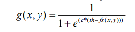
where :

g (x,y) is Enhanced pixel value

c is the Contrast factor

th is the Threshold value

fs(x,y) is original image

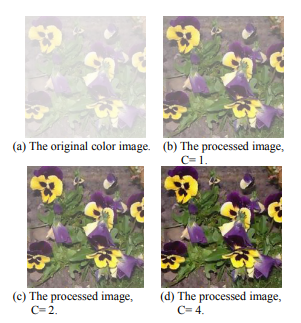
Now, Here the hyperparameter is “c” and “th”. By adjusting them we will able to control the overall contrast enhancement by lightening and darkening.

Conclusion

In this article, I have explained several types of data preprocessing in machine learning. I think my work will help you in certain ways. If you suggest adding something more, Feel free to reach me. Just drop me a mail. See you next time with another blog