


Have you ever heard of the "curse of dimensionality"? It's a common problem in machine learning where datasets with too many features can become too complex for algorithms to handle effectively. That is where Principal Component Analysis (PCA) comes in. PCA is a powerful tool that allows data scientists to reduce the dimensionality of large datasets, while maintaining the integrity of the underlying structure. But PCA isn't just useful for machine learning. It has a range of practical applications, from image processing and signal analysis to finance and genomics. In this article, we will be exploring what it is, how it works, and why it is such an essential technique in modern data science. So whether you are a seasoned data scientist or just starting your journey, let us get ready to unravel the mysteries of Principal Component Analysis.
What is principal component analysis?
Principal Component Analysis (PCA) is a statistical method that is used to reduce the dimensionality of large datasets. PCA is also considered as a mathematical technique that transforms a dataset into a new coordinate system in such a way that the first axis, called the principal component, captures the maximum amount of variance in the data. The second principal component captures the next highest variance, and so on.
The goal of PCA is to find a reduced set of variables that can explain the maximum amount of variance in the original data. It is a popular technique in machine learning and data analysis for identifying the underlying structure in data and extracting the most relevant features.
Also, it can improve the accuracy and efficiency of machine learning models by removing redundant features and reducing noise in the data. Finally, PCA can also help to visualize high-dimensional data in two or three dimensions, making it easier to interpret and understand.
Steps Involved in Principal Component Analysis
- Standardize the data: To ensure that every feature carries equal weight in the analysis, it is necessary to standardize the data. This can be achieved by subtracting the mean from each value and dividing by the standard deviation.
- Compute the covariance matrix: We need to compute the covariance matrix of the standardized data. This matrix represents the relationships between each feature in the dataset.
- Compute the eigenvectors and eigenvalues: We use the covariance matrix to compute the eigenvectors and eigenvalues. The eigenvectors represent the principal components, and the eigenvalues represent the variance explained by each principal component.
- Select the number of principal components: We need to decide how many principal components we want to keep. We perform this by looking at the percentage of variance explained by each component and choosing the components that explain the most variance.
- Project the data onto the new coordinate system: We use the selected principal components to transform the data into new coordinates where each data point is represented by its principal component scores.
Principal Component Analysis using Python
We will examine each step of implementing PCA in a single class in detail. The skeleton class below can serve as a blueprint.
class PCA:
   def fit_transform(self, X, n_components=2):
       pass
   def standardize_data(self, X):
       pass
   def get_covariance_matrix(self):
       pass
 def get_eigenvectors(self, C):
       pass
   def project_matrix(self, eigenvectors):
       pass
Step 1: Standardize the data
In order to standardize the variables to the same scale, we use the following formula.
Z = (Value- Mean)/Standard Deviation
Where,
Mean = Sum of Terms/Total Number of Terms
Step2: Compute the covariance matrix
The covariance matrix indicates the extent to which two random variables vary together. If the covariance is positive, the two variables are correlated, meaning they move in the same direction (i.e., increase or decrease together). Conversely, if the covariance is negative, the variables are inversely correlated, moving in opposite directions (e.g., one increases while the other decreases).
Suppose we have a dataset with three features. If we compute the covariance matrix, we will obtain a 3x3 matrix that displays the covariance of each column with all other columns and itself.
The covariance matrix plays a crucial role in the eigendecomposition step of PCA. It helps us choose the main directions or vectors that explain most of the variance in the dataset. To compute the covariance matrix, we use a formula that involves mean-centering our data.
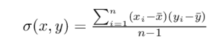
covariance matrix
Where
If the data is already mean-centered, we can simplify the formula by expressing it as a dot product of the data matrix with itself divided by the number of samples.
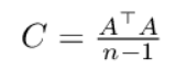
dot product formula
We shall now implement our first two class methods.
class PCA:
   def standardize_data(self, X):
       # subtract mean and divide by standard deviation columnwise
       numerator = X - np.mean(X, axis=0)
       denominator = np.std(X, axis=0)
       return numerator / denominator

   def get_covariance_matrix(self, ddof=0):
       # calculate covariance matrix with standardized matrix A
       C = np.dot(self.A.T, self.A) / (self.n_samples-ddof)
       return C
Step3: Compute the eigenvectors and eigenvalues:
In the next step of our implementation, we focus on decomposing the covariance matrix. Eigendecomposition involves breaking down a matrix into its eigenvectors and eigenvalues. Eigenvectors provide information about the data direction, while eigenvalues can be seen as coefficients indicating how much variance each eigenvector carries. By decomposing our covariance matrix, we obtain the eigenvectors that explain the maximum variance in our dataset, which we can then use to project the original matrix into a lower dimension.
Fortunately, we can use NumPy's built-in function to decompose the covariance matrix. Computing the eigenvectors and eigenvalues manually is quite complicated.
Step4: Select the number of principal components
The only thing we need to do is sort the eigenvalues and eigenvectors based on the number of components we specify to select the most important eigenvectors.
Let us implement the above two steps
class PCA:
    #...
def get_eigenvectors(self, C):
    # calculate eigenvalues & eigenvectors of covariance matrix 'C'
    eigenvalues, eigenvectors = np.linalg.eig(C)

    # sort eigenvalues descending and select columns based on n_components
    n_cols = np.argsort(eigenvalues)[::-1][:self.n_components]
    selected_vectors = eigenvectors[:, n_cols]
    return selected_vectors
Step5: Project the data onto the new coordinate system:
After selecting the most significant eigenvectors, we can now project the initial matrix into a lower-dimensional space. We accomplish this by performing a dot product between the matrix and the eigenvectors, which can also be viewed as a basic linear transformation.
After implementing the above steps our final code will be this
class PCA:

    def standardize_data(self, X):
        # subtract mean and divide by standard deviation columnwise
        numerator = X - np.mean(X, axis=0)
        denominator = np.std(X, axis=0)
        return numerator / denominator

    def get_covariance_matrix(self, ddof=0):
        # calculate covariance matrix with standardized matrix A
        C = np.dot(self.A.T, self.A) / (self.n_samples-ddof)
        return C

    def get_eigenvectors(self, C):
        # calculate eigenvalues & eigenvectors of covariance matrix 'C'
        eigenvalues, eigenvectors = np.linalg.eig(C)
        # sort eigenvalues descending and select columns based on n_components
        n_cols = np.argsort(eigenvalues)[::-1][:self.n_components]
        selected_vectors = eigenvectors[:, n_cols]
        return selected_vectors

 def fit_transform(self, X, n_components=2):
        # get number of samples and components
        self.n_samples = X.shape[0]
        self.n_components = n_components
        # standardize data
        self.A = self.standardize_data(X)
        # calculate covariance matrix
        covariance_matrix = self.get_covariance_matrix()
        # retrieve selected eigenvectors
        eigenvectors = self.get_eigenvectors(covariance_matrix)
        # project into lower dimension
        projected_matrix = self.project_matrix(eigenvectors)
        return projected_matrix


    def project_matrix(self, eigenvectors):
        P = np.dot(self.A, eigenvectors)
        return P
Now that we have created our class for PCA. Let us now implement it with an example dataset we shall use the iris dataset, which comprises of 150 data points with 4 different features or variables (Sepal Length, Sepal Width, Petal Length, Petal Width).
We shall now instantiate our own PCA class and fit it on the dataset.
from sklearn import datasets

# load iris dataset
iris = datasets.load_iris()
X = iris.data
y = iris.target

# instantiate and fit_transform PCA
pca = PCA()
X_pca = pca.fit_transform(X, n_components=2)

# plot results
fig, ax = plt.subplots(1, 1, figsize=(10,6))

sns.scatterplot(
    x = X_pca[:,0],
    y = X_pca[:,1],
    hue=y
)

ax.set_title('Iris Dataset')
ax.set_xlabel('PC1')
ax.set_ylabel('PC2')

sns.despine()
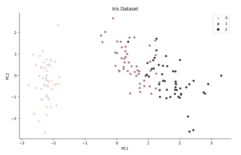
output
Through the application of PCA, we were able to disentangle some of the class relationships and create a clearer separation between the data points. With this lower-dimensional representation, any subsequent classification task would likely become much simpler.
| Advantages of PCA | Disadvantages of PCA |
|---|---|
| Reduces the dimensionality of large datasets | Can be sensitive to outliers |
| Simplifies data and removes redundant information | Requires prior knowledge of data structure and scaling |
| Improves algorithm performance and efficiency | Can be difficult to interpret and explain to non-technical stakeholders |
| Visualizes complex data in a simpler way | May result in loss of important information |
| Can be combined with other machine learning techniques | Assumes linear relationships between variables |
| Can handle highly correlated variables effectively | May not work well with categorical variables |
Conclusion
Principal Component Analysis (PCA) is a powerful dimensionality reduction technique in machine learning that has several advantages. PCA can effectively reduce the number of features in a dataset, making it easier to analyze and interpret while also reducing the potential for overfitting. It can also help identify important features in a dataset and aid in visualizing data in a lower-dimensional space.
However, PCA is not without limitations. Sometimes it can be sensitive to outliers and may not always be appropriate for all types of data. Additionally, there are other factor analysis methods that may be suitable for certain types of datasets.
Overall, PCA is a valuable tool in machine learning, but its use should be carefully considered and compared to other techniques depending on the specific needs of the analysis.
For more such Insightful blogs you can also read our other articles.


