Probability Distributions in Statistics

This is the continuation of my first part where our main focus here is on understanding the important probability distributions and some related underlying concepts behind modelling distributions of data.

Without further ado, let us cut to the chase.

Important Discrete Distributions

Uniform Distribution:

Let’s consider of a sample space: S = {1,2,3…k}. Uniform distribution holds equal probabilities which x can take. The outcomes are equally likely to occur(ex- tossing a coin) and we can equal assignment(1/k) to all outcomes.

Distribution: P(X=x) = 1/k, which is the pdf of X. From this we can infer that more the no of elements , the more is the variance in the sample.

Bernoulli Distribution:

A Bernoulli trial is an experiment which has (or can be regarded as having) only two possible outcomes — s (“success”) and f (“failure”).

In short, we can say there’s 1 experiment with n trials called the sequence of n independent B trials. For example, tossing 3 coins simultaneously will be a sequence of 3 B trials together and trials are identical that is for each trial P({S})=θ. The trials are independent and identically distributed.

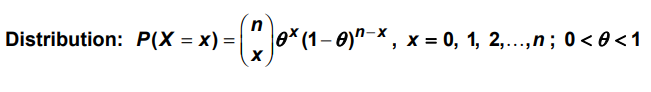
Binomial Distribution:

In Binomial distribution, we use two parameters (n,θ) and let S be a sample space which is the joint set of outcomes of n trials. n will be 3 for a sample space of tossing 3 coins simultaneously. The trials are independent of one another, the outcome of any trial does not depend on the outcomes of any other trials. Let’s have a look at the distribution function:

Geometric Distribution:

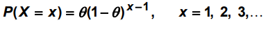
In geometric Binomial distribution we usually end the experiment whenever there’s a first success. Here the random variable X is the no of trials on which first success occurs. Imagine of a experiment of tossing a coin whenever a head occurs. The values can be countably infinite since we don’t know when the success will occur and it can go till infinite times.

For X =x, there must be a run of (x-1) failures followed by a success. So, the distribution looks like:

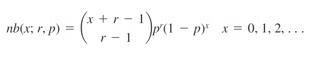
Negative Binomial Distribution:

It is the special case of geometric Binomial distribution. In negative Binomial distribution the number of trials(n) is not fixed as in normal Binomial. In normal Binomial distribution we see the no of failures that counts before a success. The experiment continues (trials are performed) until a total of r successes have been observed. The PDF of a normal Binomial distribution is given by:

Poisson Distribution:

Let’s go with an example, If we know on an average(across years) at a particular cross section, 30 vehicles pass by in a minute. So, what is the probability that 50 or 100 vehicles will pass by in 1 minute (based on past records)? well, this can be modelled by a Poisson Distribution. The distribution of P(X=x) is given by:

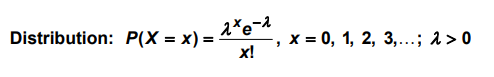
Here x can take values till infinite because we don’t know the exact no of occurrence given the past records. λ is the parameter/rate of occurrence of an event. Also note that Poisson distribution is a positively skewed distribution.

Important Continuous Distributions

So, for continuous distributions point probabilities are always zero. That is P(X=x) = 0. We’ll use P(X ≤ x) and P(X<x) interchangeably. Please note that: P(X>x) = 1-P(X<x), also P(X<x) = 1-P(X>x). Keep in mind that area under a continuous

Uniform distribution:

The Uniform Distribution (also called the Rectangular Distribution) is the simplest distribution where we have equal probabilities or the probability distribution is uniform in a range.

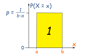
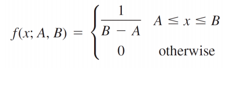
The area of the rectangle is 1 or p × (b−a) = 1. PDF of X following a uniform distribution:

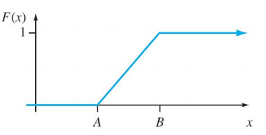
We can also generate random numbers between 0 & 1 using a uniform distribution. Well, this is how the CDF of a uniform distribution will be!

Normal Distribution:

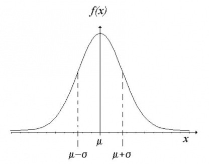
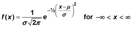
The normal distribution is probably the most important distribution in all of probability and statistics. Many populations have distributions that can be fit very closely by an appropriate normal (or Gaussian) bell-shaped curve. The tails of this distribution doesn’t touch x-axis, instead touches at -∞ to ∞ hovering above the bell shaped curve. Examples can be height, weight, marks scored follows a normal distribution.

A continuous random variable X is said to have a normal distribution with parameters µ and σ > 0. The distribution is symmetrical about µ and the pdf of X is given by:

Standard Normal Distribution:

This is a special case of Normal distribution. The normal distribution with parameter values µ = 0 and σ = 1 is called the standard normal distribution. We cannot find the explicit value of X by integrating so the distribution is provided by transforming to a Z score[(X-µ)/σ], then scaled to find the values of X.

P(X ≤ x) or P(X < x)= P(Z< (X-µ)/σ) → CDF of a Normal distribution

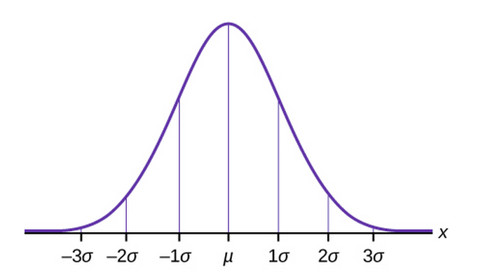
The total spread is 6σ which constitutes 3σ on the left and 3σ on right of the mean(µ).

Exponential Distribution:

X is said to have an exponential distribution with the rate parameter λ (λ > 0) if the pdf of X is:

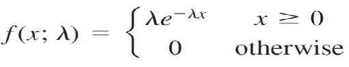
Here λ denotes the rate of occurrence/waiting time till the next event occurs. This waiting time is modelled by a exponential distribution. In simple words, waiting time between two events. Life expectancy of a light bulb is modelled by an exponential distribution in Poisson process with parameter λ.

There are many other distributions like Chi-Square, t-distribution, F-distribution and many more. There’s no way bounding ourselves from google search and exploring these vast range of topics. We could have included here but it will be an overflow of this story and already it has been extended much and there’s many new things coming up next. So please don’t hesitate to scroll down below ????

JOINTLY DISTRIBUTED RANDOM VARIABLES

It is basically the generalization of two or more random variables. We consider the typical case of two random variables that are either both discrete or both continuous. In cases where one variable is discrete and the other continuous, appropriate modifications are easily made. Suppose in a survey, apart from collecting the weights of students in a class we are interested to go with the heights of the students as well since both of them possess a relationship while calculating the heights of the students in a class. For a 2D random variable, possible value of [X1,X2] are either finite or countably infinite in number.

Joint Probability mass function for discrete Bi-variate probability distribution:

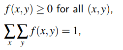
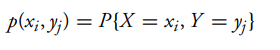
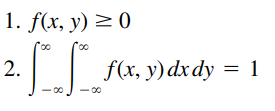
The case where both variables are continuous is obtained easily by analogy with the discrete case on replacing sums by integrals. Thus the joint probability function for the random variables X and Y (or, as it is more commonly called, the joint density function of X and Y ) is defined by:

Marginal Distribution

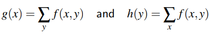
It is defined for each random variable. This is the distribution of X alone without considering the values that Y can take and vice versa. The marginal distribution of a discrete random variable X and Y alone defined by a function g(x) and h(y) is respectively:

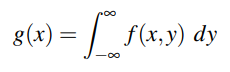
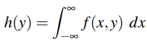
The marginal distributions(Marginal PDF) of X alone and Y alone for a continuous case are respectively:

Independent Random Variables

The random variables X and Y are said to be independent if for any two sets of real numbers A and B is: P{X ∈ A, Y ∈ B} = P{X ∈ A}*P{Y ∈ B}

When X and Y are discrete random variables, the condition of independence is given by: p(x, y) = p(x)*p(y) for all x, y.

In the jointly continuous case, the condition of independence is equivalent to: f(x, y) = f(x)*f(y)

Conditional Probability Density Function (Conditional PDF)

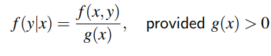
The relationship between two random variables can often be clarified by consideration of the conditional distribution of one given the value of the other. The conditional distribution of Y|X = x is:

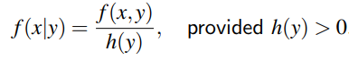
Similarly, the conditional distribution of X|Y = y is:

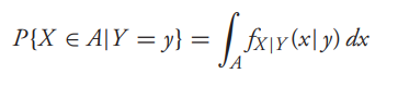
Now, if X and Y are jointly continuous, then, for any set A:

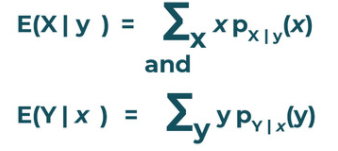
Conditional Expectation for discrete case:

Most often we are interested in finding out the weight of a person given the height of the person. Generally we want to find the expected value of X given Y. If [X,Y] is a discrete random vector, the conditional expectations are:

For continuous case:

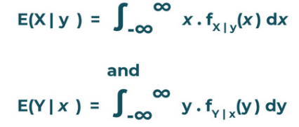
Alternatively this function E(X | y) is also known as Regression of Mean. The graph of this function is called the regression of X on Y or how the expectation of X varies with y.

Covariance & Correlations

The degree of association between X & Y determines how associated these variables or the variations are. Covariance determines the direction of linear relationship between 2 variables, whereas a related quantity to covariance is Correlation which determines the strength of the relationship between X and Y. Covariance & Correlation is calculated respectively by:

Cov(X,Y) = E[XY]-E[X]*E[Y] and,

Corr(X,Y) = Cov(X,Y)/sqrt(Var(X)*Var(Y))

Covariance is positive if X ∝ Y, negative if X ∝ 1/Y or vice-versa interchangeably. If the correlation(ρ) comes out to be 1, it signifies that X & Y are 100% correlated. The correlation coefficient takes a value in the range -1≤ρ≤1.

End Notes

We are almost on the finishing line. Let me tell you, statistics as a whole is a vast area and there’s no end to this massive sea. We might end up doing a PHD in statistics if we were to master each of its counterparts. In this article, I have tried my best to frame the important ones starting from random variables(discussed in part1), went through some major probability distributions and concepts which one can have to build your toolkit as a statistician and derive meaningful insights!

Thankyou for reading. Please share your feedbacks incase you really enjoyed spending few time over these two parts of my detailed story!