As Josh Wills once said, “Data Scientist is a person who is better at statistics than any programmer and better at programming than any statistician.”

Hi Guys, my name is Shirsh and I am a aspiring Data Scientist ,currently I am building my skill sets to excel in this domain , in this blog I will be summarizing all important Statistics Concept which I have learnt till date. Doing this will help me build my concept better and would also help guys who are new to this field.

So let’s get started

What do I mean when I say what is Probability?

1.There is 50% chance of rains tomorrow evening

2. There in .33 probability of you failing

_Probability in simple words means : Unable to predict the outcomes, but in the long-run, the outcomes exhibit statistical regularity. _

Example:

Tossing a fair coin — outcomes S ={Head, Tail} Unable to predict on each toss whether is Head or Tail. In the long run can predict that 50% of the time heads will occur and 50% of the time tails will occur.

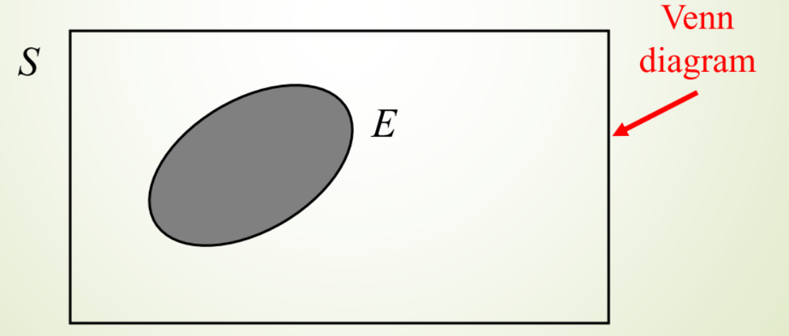
The sample Space, S The sample space, S, for a random phenomena is the set of all possible outcomes.

Event , E The event, E, is any subset of the sample space, S. i.e. any set of outcomes (not necessarily all outcomes) of the random phenomena

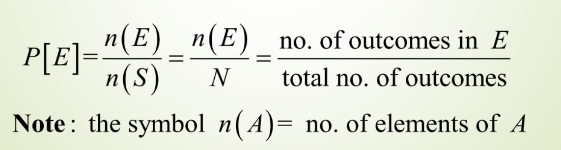
Definition: probability of an Event E.

Suppose that the sample space S = {o1, o2, o3, … oN} has a finite number, N, of outcomes. Also each of the outcomes is equally likely (because of symmetry). Then for any event E

If two events A and B are are mutually exclusive then:

• They have no outcomes in common. They can’t occur at the same time. The outcome of the random experiment can not belong to both A and B.

Conditional Probability

1. Frequently before observing the outcome of a random experiment you are given information regarding the outcome
2. How should this information be used in prediction of the outcome.
3. Namely, how should probabilities be adjusted to take into account this information
4. Usually the information is given in the following form: You are told that the outcome belongs to a given event. (i.e. you are told that a certain event has occurred)

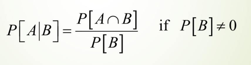
Definition

Suppose that we are interested in computing the probability of event A and we have been told event B has occurred. Then the conditional probability of A given B is defined to be:

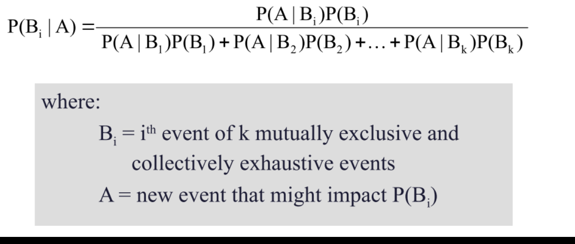
Bayes’ Theorem

Bayes’ Theorem is used to revise previously calculated probabilities based on new information. Developed by Thomas Bayes in the 18th Century. It is an extension of conditional probability.

Random Variable

A numerical outcome of any random phenomenon is called an Random Variable.

A random variable x takes on a defined set of values with different probabilities.

• For example, if you roll a die, the outcome is random(not fixed) and there are 6 possible outcomes, each of which occur with probability one-sixth.
• For example, if you poll people about their voting preferences, the percentage of the sample that responds “Yes on Proposition 100” is a also a random variable (the percentage will be slightly differently every time you poll)

Random variables can be discrete or continuous

Discrete random variables have a countable number of outcomes

• Examples: Dead/alive, treatment/placebo, dice, counts,etc.

Continuous random variables have an infinite continuum of possible values.

• Examples: blood pressure, weight, the speed of a car, the real numbers from 1 to 6.

Probability functions

A probability function maps the possible values of x against their respective probabilities of occurrence, p(x) p(x) is a number from 0 to 1.0. The area under a probability function is always 1.

Types of Probability function: There are mainly three types of functions

Probability Mass Function (PMF)

The Probability Mass Function (PMF) also called a probability function or frequency function which characterizes the distribution of a discrete random variable. Let X be a discrete random variable of a function, then the probability mass function of a random variable X is given by

Px (x) = P( X=x ), For all x belongs to the range of X

It is noted that the probability function should fall on the condition :

Px (x) ≥ 0 and ∑xϵRange(x) Px (x) = 1

Here the Range(X) is a countable set and it can be written as { x1, x2, x3, ….}. This means that the random variable X takes the value x1, x2, x3, ….

** Cumulative Distribution Function (CDF)**

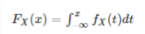
The Cumulative Distribution Function (CDF), of a real-valued random variable X, evaluated at x, is the probability function that X will take a value less than or equal to x. It is used to describe the probability distribution of random variables in a table. And with the help of these data, we can create a CDF plot in excel sheet easily.

In other words, CDF finds the cumulative probability for the given value. To determine the probability of a random variable, it is used and also to compare the probability between values under certain conditions. For discrete distribution functions, CDF gives the probability values till what we specify and for continuous distribution functions, it gives the area under the probability density function up to the given value specified. In this article, we are going to discuss the formulas, properties and examples of the cumulative distribution function.

The CDF defined for a discrete random variable is given as

Fx(x) = P(X≤x)

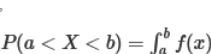
Where X is the probability that takes a value less than or equal to x and that lies in the semi-closed interval (a,b], where a < b.

Therefore the probability within the interval is written as

P(a < X ≤ b)=Fx(b)-Fx(a)

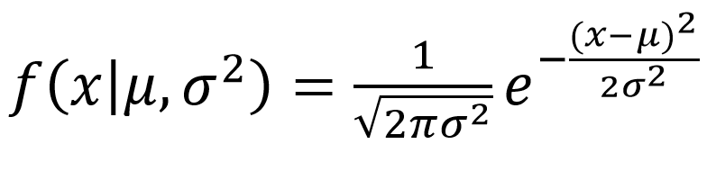
Probability Density Function (PDF)

Probability Density Function (PDF) is used to define the probability of the random variable coming within a distinct range of values, as objected to taking on anyone value. The probability density function is explained here in this article to clear the concepts of the students in terms of its definition, properties, formulas with the help of example questions. The function explains the probability density function of normal distribution and how mean and deviation exists. The standard normal distribution is used to create a database or statistics, which are often used in science to represent the real-valued variables, whose distribution are not known.

NOTE :PDF is defined for continuous random variables whereas PMF is defined for discrete random variables.

for inline plots in jupyter

%matplotlib inline

import matplotlib

import matplotlib.pyplot as plt

for latex equations

from IPython.display import Math, Latex

for displaying images

from IPython.core.display import Image

import seaborn

import seaborn as sns

settings for seaborn plotting style

sns.set(color_codes=True)

settings for seaborn plot sizes

sns.set(rc={‘figure.figsize’:(5,5)})

1. Uniform Distribution

Perhaps one of the simplest and useful distribution is the uniform distribution. The probability distribution function of the continuous uniform distribution is:

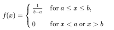
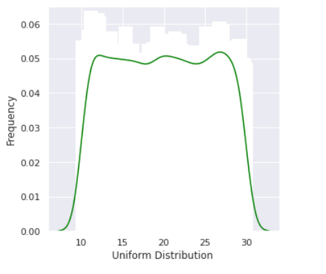
Since any interval of numbers of equal width has an equal probability of being observed, the curve describing the distribution is a rectangle, with constant height across the interval and 0 height elsewhere. Since the area under the curve must be equal to 1, the length of the interval determines the height of the curve. The following figure shows a uniform distribution in interval (a,b). Notice since the area needs to be 1. The height is set to 1/(b−a).

import uniform distribution

from scipy.stats import uniform

random numbers from uniform distribution

n = 10000 start = 10 width = 20 data_uniform = uniform.rvs(size=n, loc = start, scale=width) ax = sns.distplot(data_uniform, bins=100, kde=True, color=’green’, hist_kws={“linewidth”: 15,’alpha’:1}) ax.set(xlabel=’Uniform Distribution ‘, ylabel=’Frequency’)

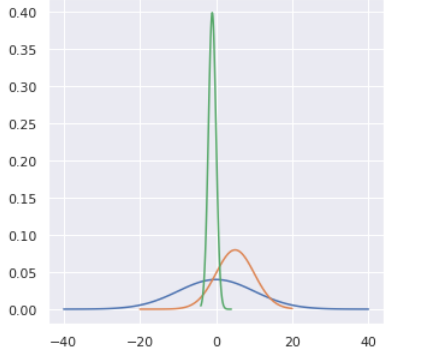
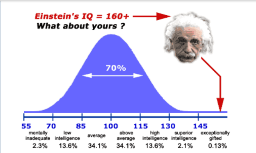
2. Normal Distribution

Normal Distribution, also known as Gaussian distribution, is ubiquitous in Data Science. We will encounter it at many places especially in topics of statistical inference. It is one of the assumptions of many data science algorithms too.

alternative code

import matplotlib.pyplot as plt import numpy as np import scipy.stats as stats import math

mu = 0 # mean variance = 100 sigma = math.sqrt(variance) # sigma is standard deviation x = np.linspace(mu — 4_sigma, mu + 4_sigma, 100) x1 = np.linspace(mu — 4_5, mu + 4_5, 100) x2 = np.linspace(mu — 4_1, mu + 4_1, 100) plt.plot(x, stats.norm.pdf(x, 0, sigma)) plt.plot(x1, stats.norm.pdf(x1, 5, 5)) plt.plot(x2, stats.norm.pdf(x2, -1, 1))

plt.show()

3. Poisson Distribution

Poisson random variable is typically used to model the number of times an event happened in a time interval. For example, the number of users visited on a website in an interval can be thought of a Poisson process. Poisson distribution is described in terms of the rate (μ) at which the events happen. An event can occur 0, 1, 2, … times in an interval. The average number of events in an interval is designated λ (lambda). Lambda is the event rate, also called the rate parameter. The probability of observing k events in an interval is given by the equation :

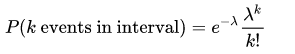
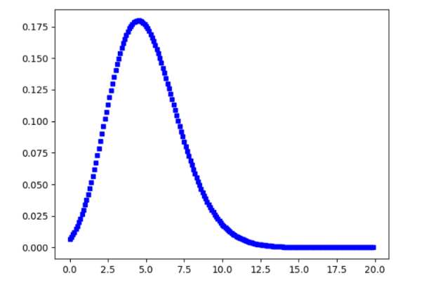
From the above we can say that this Poisson distribution is forming a Bell curved shape and hence can also be called as a Discrete Normal Distribution

Probability of Multiple Random Variables

In machine learning, we are likely to work with many random variables. For example, given a table of data, such as in excel, each row represents a separate observation or event, and each column represents a separate random variable. Variables may be either discrete, meaning that they take on a finite set of values, or continuous, meaning they take on a real or numerical value. As such, we are interested in the probability across two or more random variables. This is complicated as there are many ways that random variables can interact, which, in turn, impacts their probabilities. This can be simplified by reducing the discussion to just two random variables (X, Y), although the principles generalize to multiple variables. And further, to discuss the probability of just two events, one for each variable (X=A, Y=B), although we could just as easily be discussing groups of events for each variable. Therefore, we will introduce the probability of multiple random variables as the probability of event A and event B, which in shorthand is X=A and Y=B. We assume that the two variables are related or dependent in some way.

As such, there are three main types of probability we might want to consider; they are:

• Joint Probability: Probability of events A and B.
• Marginal Probability: Probability of event X=A given variable Y.
• Conditional Probability: Probability of event A given event B.

Joint Probability

The probability of two (or more) events is called the joint probability. The joint probability of two or more random variables is referred to as the joint probability distribution.

For example, the joint probability of event A and event B is written formally as:

• P(A and B)
• This can be stated as P(A and B) = P(A given B) * P(B)
• The joint probability is symmetrical, meaning that P(A and B) is the same as P(B and A). The calculation using the conditional probability is also symmetrical, for example:
• P(A and B) = P(A given B) * P(B) = P(B given A) * P(A)

Marginal Probability

We may be interested in the probability of an event for one random variable, irrespective of the outcome of another random variable.

The probability of one event in the presence of all (or a subset of) outcomes of the other random variable is called the marginal probability or the marginal distribution. The marginal probability of one random variable in the presence of additional random variables is referred to as the marginal probability distribution.

Its formula is given by P(X=A) = summation P(X=A, Y=y_i) for all y and a fixed X=A

Descriptive Statistics

Descriptive Statistics are Used by Researchers to Report on Populations and Samples

• In Sociology: Summary descriptions of measurements (variables) taken about a group of people
• By Summarizing Information, Descriptive Statistics Speed Up and Simplify Comprehension of a Group’s Characteristics

What Are Descriptive Statistics?

Descriptive statistics are brief descriptive coefficients that summarize a given data set, which can be either a representation of the entire or a sample of a population. Descriptive statistics are broken down into measures of central tendency and measures of variability (spread). Measures of central tendency include the mean, median, and mode, while measures of variability include standard deviation, variance, minimum and maximum variables, kurtosis, and skewness.

Measures of Central Tendency

• Example to compute the Measures of Central Tendency

Consider the following data points.

17, 16, 21, 18, 15, 17, 21, 19, 11, 23

• Mean — Mean is calculated
• Median — To calculate Median, lets arrange the data in ascending order.
• 11, 15, 16, 17, 17, 18, 19, 21, 21, 23

Since the number of observations is even (10), median is given by the average of the two middle observations (5th and 6th here).

• Mode — Mode is given by the number that occurs maximum number of times. Here, 17 and 21 both occur twice. Hence, this is a Bimodal data and the modes are 17 and 21.

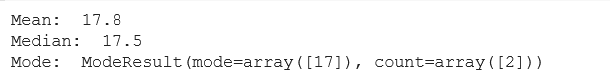
Using Python we can achieve all of this in a seconds

import numpy as np from scipy import stats

dataset= [17, 16, 21, 18, 15, 17, 21, 19, 11, 23]

#mean value mean= np.mean(dataset)

#median value median = np.median(dataset)

#mode value mode= stats.mode(dataset)

print(“Mean: “, mean) print(“Median: “, median) print(“Mode: “, mode)

Measures of Dispersion (or Variability)

Measures of Dispersion describes the spread of the data around the central value (or the Measures of Central Tendency)

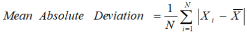
• Absolute Deviation from Mean — The Absolute Deviation from Mean, also called Mean Absolute Deviation (MAD), describe the variation in the data set, in sense that it tells the average absolute distance of each data point in the set. It is calculated as

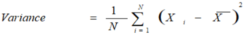
• Variance — Variance measures how far are data points spread out from the mean. A high variance indicates that data points are spread widely and a small variance indicates that the data points are closer to the mean of the data set. It is calculated as

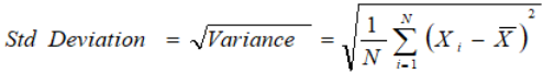
• Standard Deviation — The square root of Variance is called the Standard Deviation. It is calculated as

• Range — Range is the difference between the Maximum value and the Minimum value in the data set. It is given as

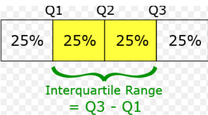
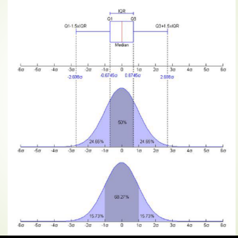
• Quartiles — Quartiles are the points in the data set that divides the data set into four equal parts. Q1, Q2 and Q3 are the first, second and third quartile of the data set.
• 25% of the data points lie below Q1 and 75% lie above it.
• 50% of the data points lie below Q2 and 50% lie above it. Q2 is nothing but Median.
• 75% of the data points lie below Q3 and 25% lie above it.

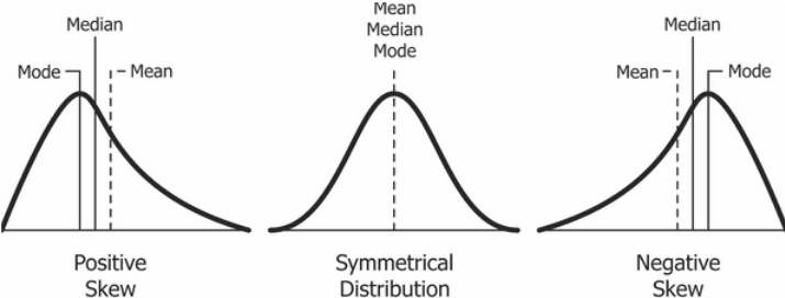
• Skewness — The measure of asymmetry in a probability distribution is defined by Skewness. It can either be positive, negative or undefined.
• Positive Skew — This is the case when the tail on the right side of the curve is bigger than that on the left side. For these distributions, mean is greater than the mode.
• Negative Skew — This is the case when the tail on the left side of the curve is bigger than that on the right side. For these distributions, mean is smaller than the mode.

The most commonly used method of calculating Skewness is

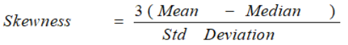
If the skewness is zero, the distribution is symmetrical. If it is negative, the distribution is Negatively Skewed and if it is positive, it is Positively Skewed.

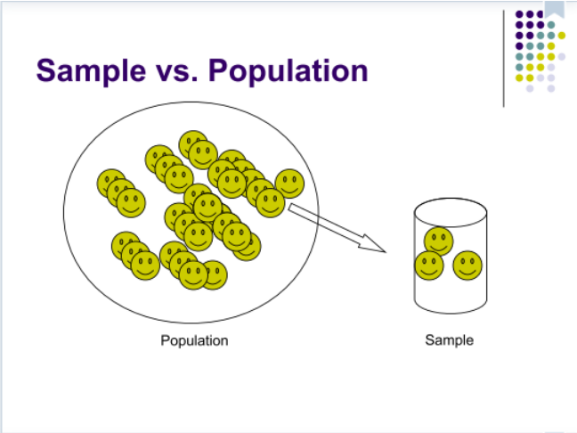
Statistical inference

The fundamental idea is to use data from a sample to infer information about the population. What I mean is, it’s impractical to actually evaluate whole of the population, so instead take a small sample of the population that effectively can represent the whole population.

For example, in a drug testing scenario, you will select a group of people or subjects such that almost equal representation exists, one on whom the new drug is being tested and one whom the old drug is being tested in order to compare.

To sum up

The process of making guess/inference about the truth from a sample is called Statistical Inference

Central Limit Theorem

• In probability theory, the central limit theorem (CLT) establishes that, in some situations, when independent random variables are added, their properly normalized sum tends toward a normal distribution(informally a “bell curve”) even if the original variables themselves are not normally distributed.
• Suppose that a sample is obtained containing a large number of observations, each observation being randomly generated in a way that does not depend on the values of the other observations, and that the arithmetic mean of the observed values is computed.

If this procedure is performed many times, the central limit theorem says that the distribution of the average will be closely approximated by a normal distribution. A simple example of this is that if one flips a coin many times the probability of getting a given number of heads in a series of flips will approach a normal curve, with mean equal to half the total number of flips in each series. (In the limit of an infinite number of flips, it will equal a normal curve.)

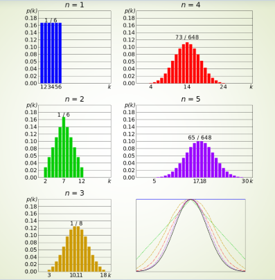
When the coins are flipped for a very large n number of times distribution of number of heads associated with each throw has started to show a Bell Curve which approximately looks like and normal distribution.

Interval Estimation

• Population Mean: µ Known
• Population Mean: µ Unknown
• Population Std Dev: σ Unknown
• Determining the Sample Size
• Population Proportion

Basic Intuition

• In CLT we plot a graph with sample means VS frequency of the means
• Here sample mean is a Random variable on x axis with its respective frequency on y axis
• Sample means here is expectation value of n random samples chosen

Margin of Error and Interval Estimate

• A point estimator cannot be expected to provide the exact value of the population parameter
• An interval estimate can be computed by adding and subtracting a margin of error to the point estimate

Point Estimate +/- Margin of Error

• The purpose of an interval estimate is to provide information about how close the point estimate is to the value of the parameter.
• In order to develop an interval estimate of a population mean, the margin of error must be computed using either: the population standard deviation σ , or the sample standard deviation s
• σ is rarely known exactly, but often a good estimate can be obtained based on historical data or other information.
• We refer to such cases as the σ known case.

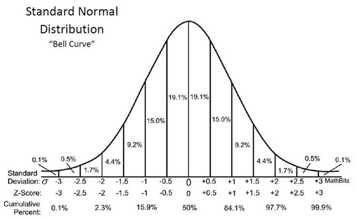
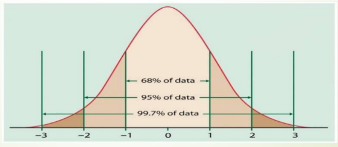
Z-distribution

In statistics, the Z-distribution is used to help find probabilities and percentiles for regular normal distributions (X). It serves as the standard by which all other normal distributions are measured. The Z-distribution is a normal distribution with mean zero and standard deviation 1

Interval Estimate of a Population Mean

After we found a point estimate of the population mean, we would need a way to quantify its accuracy. Here, we discuss the case where the population variance σ2 / std deviation σ is assumed known

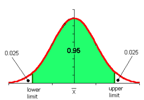
Meaning of Confidence

• Because 90% of all the intervals constructed using Xmean ± 1.645 σ will contain the population mean, we say we are 90% confident that the interval contains the population mean µ.
• We say that this interval has been established at the 90% confidence level.
• The value .90 is referred to as the confidence coefficient.
• Similarly 95% Confidence Interval (C.I.) means Xmean ± 1.96 σ will contain the population mean µ

Thanks! for reading.