The Game of Random Variables

What is a Random Variable ?

As the name suggests, it is a term that associates itself to the concept of randomness and uncertainty. There are numerous such incidents that occur in our day-to-day life whose outcomes are difficult to predict with utmost certainty. For example, while playing a game of basket ball, the certainty with which you put the ball in the basket from the half line depends on your expertise in the game. Similarly, you can’t accurately guess the number of likes you might get in your next Instagram post. It has to depend on a wide range of factors such as visual appeal, message in the caption, and your brand/product outreach.

Here the phrase ‘number of likes on next Instagram post’ can be coined as a random variable. The number of likes on a given post is a variable that can take any random integer value starting from 0 till infinity. Although the probability of you getting likes anything greater than 10000 might be bleak if you are a small brand. The probability of you having 5 billion likes is essentially 0 even if you are the largest brand in the world since the current population of the world is 7.9 billion and more than half of the world population is not on the internet and especially not on Instagram. Similarly, the total number of likes on a decent post not crossing 10 likes might be bleak as well, if your account has at least 100 followers.

Probability Distributions

We can clearly infer from the above experiment that, the probabilities of number of likes taking certain value widely varies over the entire range of random variables. And this distribution of probabilities over the entire range of values for the random variable is known as Probability Distribution of the random variable.

1. Discrete Distributions

These kind of distributions describe the variation of probabilities with respect to discrete number of countable values for the random variable. For example, when we roll a die, we have only six outcomes : 1, 2, 3, 4, 5 and 6. If our random variable is the number appearing on a rolling die, we have only six discrete values for our random variable. And probability of each of those value is 1/6, given its an unbiased die. This type of discrete distribution where all probabilities are same is also known as uniform discrete distribution.

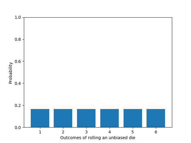
(i) Uniform discrete distribution

A uniform discrete distribution comprises of probabilities that are equal for all the values that a random variable can take. Probabilities for the outcomes of rolling an unbiased die is a classic example of uniform discrete distribution, where each of the outcomes 1, 2, 3, 4, 5 and 6 has a probability 1/6 to occur.

If we have k outcomes for a random variable X, probability of getting an outcome x is given by :

import numpy as np

import matplotlib.pyplot as plt

y = np.full(6, 1/6)

plt.bar(range(1,len(y)+1), y)

plt.ylim(0,1.)

plt.ylabel(‘Probability’)

plt.xlabel(‘Outcomes of rolling an unbiased die’)

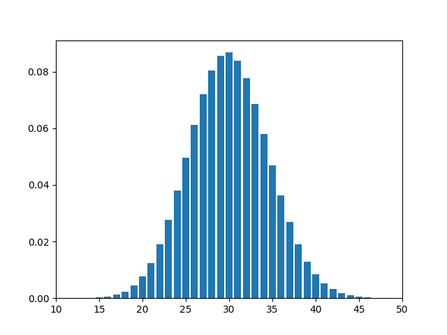
(ii) Binomial Distribution

This distribution is based on the concept of n independent and identical bernouli trials. A bernouli trial consists of two outcomes : ‘success’ and ‘failure’. In a given trial, let the probability of getting a a success in be p and probability of getting a failure is 1-p. We conduct n such trials that are independent of each other. We now want the probability of getting x number of successes in those n trials. The probability is given by :

def factorial(n):

if n > 0:

return n*factorial(n-1)

return 1

n,p = 100, 0.3

x = np.arange(0,n+1,1,dtype=int)

y = []

for x_ in x:

x_ = int(x_)

y.append( (factorial(n)/factorial(x_)/factorial(n-x_)) * ((1-p)(n-x_)) * px_ )

plt.bar(x,y)

plt.xlim(10,50)

plt.show()

A typical binomial distribution with n= 100 and p =0.3, looks like :

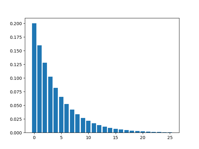
(iii) Geometric Distribution

This distribution models the number of trials on which the first success occurs. If probability of success in a given trial is p, the probability distribution of x number of such trials is given by :

n,p = 25, 0.2

x = np.arange(0,n+1,1,dtype=int)

y = (1-p)**x * p

plt.bar(x, y)

plt.show()

A geometric distribution with p = 0.2 looks like :

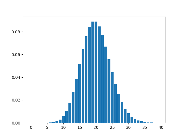
(iv) Poisson Distribution

A Poisson distribution is defined as :

where X is the random variable that determines the number of occurrences of certain event in a time interval, and λ is the average number of occurrences of certain invent in a time interval.

lamda = 20

x = np.arange(0,40,1,dtype=int)

y = []

for x_ in x:

x_ = int(x_)

y.append(lamda**x_*np.exp(-lamda)/factorial(x_))

plt.bar(x,y)

plt.show()

A poisson distribution with λ = 20 looks like :

1. Continuous Distributions

A continuous distribution is a probability distribution function for a continuous random variable i.e. a random variable with infinitely many possible values between any two random variable values. For example the height or weight of a person can be considered as a continuous random variable, whereas the probability of a person having certain height/weight gives rise to the concept of continuous probability distribution.

(i) Normal Distribution

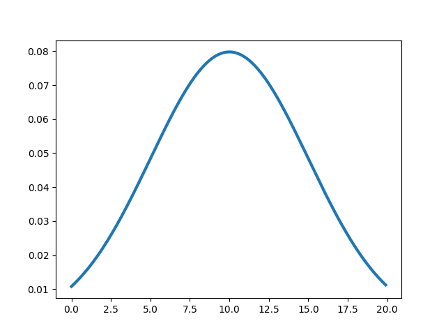
This distribution has lot of applications in statistics. It has two important parameter μ and σ, μ represents mean of the distribution, while σ represents the standard deviation of the distribution. Now the normal distribution is defined as :

mu, sig = 10, 5

x = np.arange(0,20,.1)

y = 1/(sig_np.sqrt(2_np.pi)) * np.exp(-(x-mu)2/(2*sig2))

plt.plot(x,y,linewidth=3)

plt.show()

A normal distribution with μ = 10 and σ = 5, looks like :

(ii) Exponential distribution

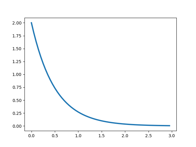
Exponential distribution is nothing but the continuous version of geometric distribution. It’s mathematical formulation is given by :

lamda = 2.

x = np.arange(0,3.,.05)

y = lamda_np.exp(-lamda_x)

plt.plot(x,y,linewidth=3)

plt.show()

Exponential distribution with λ = 2, looks like :

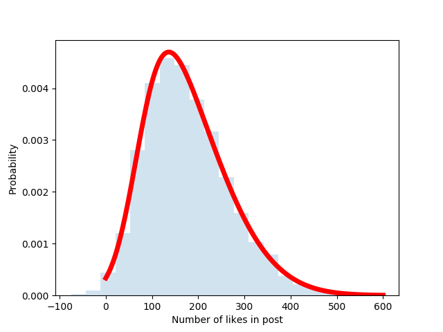
Now that we have learnt about different kind of distributions, lets try to create a possible probability distribution for the total number of likes for next Instagram post based on our earlier discussion. Suppose you are an average Instagram user with a decent 500 follower base. And you have prepared a quite engaging picture for your next Instagram post. The probability distribution for the number of likes is most likely going to be a right skewed distribution. A right skewed distribution is a distribution with most number of observations in the lower end of values for the random variable compared to those on the higher end. Similarly, a left skewed distribution is a distribution with most number of observations in the higher end of values for the random variable compared to those on the lower end.

from scipy.stats import skewnorm

a = 3

mean, std = 70, 140

fig, ax = plt.subplots(1, 1)

x = np.linspace(0,600, 200)

ax.plot(x, skewnorm.pdf(x, a, mean, std),‘r-’, lw=5)

r = skewnorm.rvs(a, mean, std, size=5000)

ax.hist(r, density=True, histtype=‘stepfilled’, alpha=0.2, bins=50)

ax.legend(loc=‘best’, frameon=False)

plt.ylabel(‘Probability’)

plt.xlabel(‘Number of likes in post’)

plt.show()

Cumulative Distribution function

Cumulative distribution function of a random variable X is defined as the sum of all the probabilities of values of X that are less than a certain value x. In mathematical terms, this can be written as:

For discrete distributions, CDF is defined as:

If f(x) is the continuous probability density function, CDF is defined as:

As x → ∞ , the cumulative distribution function P( X ≤ ∞) →1, which shows the sum of all the probabilities in a probability density function is 1.

Joint Distributions

Sometimes the probability density function is not only a function of a single variable but multiple different random variables. For example, P(X=x,Y=y) = f(x,y) is a function of two different random variables. Here f(x,y) is nothing but the Joint distribution function of both variables X and Y.

Similar to what we observed in single random variable, sum of all the probability of a joint distribution also equals 1 i.e.

Marginal Distribution

Marginal probability distribution of a variable X is defined as the probability density function with respect to X while summing the probabilities over all other variables (Y).

In case of a discrete joint distribution, marginal probability distribution is defined as:

While in case of a continuous joint distribution, marginal probability distribution is given by :

If two random variables are independent, Joint probability distribution of X and Y can be written as :

Inferential Statistics

Inferential statistics if that domain of statistics which is very useful to determine the population statistic based on a sample statistic. This technique is often used since in most real world cases, the sample size is quite smaller than the actual population and we need to determine the statistics of the population. Lets take an example to better understand the theory behind inferential statistics.

Let X be a random variable. We randomly select a sample of size n from the population. A statistic is something that is a function of n-sized sample. For example the mean and variance of the sample can be called as statistics. Again, a statistic is nothing but a random variable as well. We can randomly select a large number of such n-sized samples from the population, take mean and variances of those samples and try to see their distribution.

Sample Mean and Central Limit Theorem

Lets suppose we take large number of samples with n observations from a population having some arbitrary underlying distribution with mean μ and variance σ².

For large enough n, the sampling distribution of the sample mean resembles the normal distribution with mean μ and variance σ²/n, irrespective of underlying distribution.

This is known as Central Limit Theorem

In most cases, σ² in unknown. In those cases we can use t-distribution to approximate the distribution of sample mean. The t-distribution makes use of sample variance S² instead of population variance σ², i.e.

Sample Variance Distribution

When we try to look at the sampling distribution of sample variances, we can say that the mean of the sample variance distribution will be equal to μ. But the variance of the sampling distribution of sample variance depends on the underlying distribution of the population. However, if the underlying distribution is a normal distribution, the sampling distribution of the sample variance resembles a χ² distribution as:

Confidence Intervals

From the above discussed concepts of sampling distribution, we now will be able to estimate the parameters of the underlying distribution with certain confidence using confidence intervals. A 100(1-α) % confidence interval of the population mean is given by :

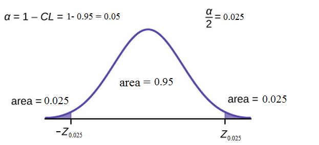
However if the standard deviation σ of underlying distribution is unknown, we can use t-statistic to come up with a confidence interval for the population mean μ, which is given by :