Understanding Time Series Analysis: Basic guide & examples

Have you ever wanted to predict the future? You may have wondered whether the stock market will go up or down tomorrow or if the demand for your company's products will increase or decrease over time. Analysis of Time series Data can help you answer these questions and more. It's a powerful tool for understanding patterns in data that change over time, and it has countless applications in fields like finance, meteorology, and marketing. We'll explore the key concepts and techniques of time series analysis and show how we can use it to gain insights and make predictions to help make better decisions. So, let's understand these concepts in more detail.

What is Time Series Analysis?

Definition: In simple terms, time series analysis is the study of a sequence of data points ordered in time. This data can be used to identify patterns, trends, and relationships over time. Examples: Weather records, economic indicators, and patient health evolution metrics

Time Series Analysis Example

Objectives: The objectives of time series analysis include understanding how variables change over time, identifying the factors that influence these changes, and predicting future values of the time series variable.

Assumptions: The only assumption in time series analysis is that the data is stationary, meaning that the statistical properties of the data are not changing over time.  More precisely, a stationary time series is one in which the mean, variance, and autocorrelation structure of the data are constant over time. This assumption ensures that the analysis is reliable and accurate.

What is Time Series?

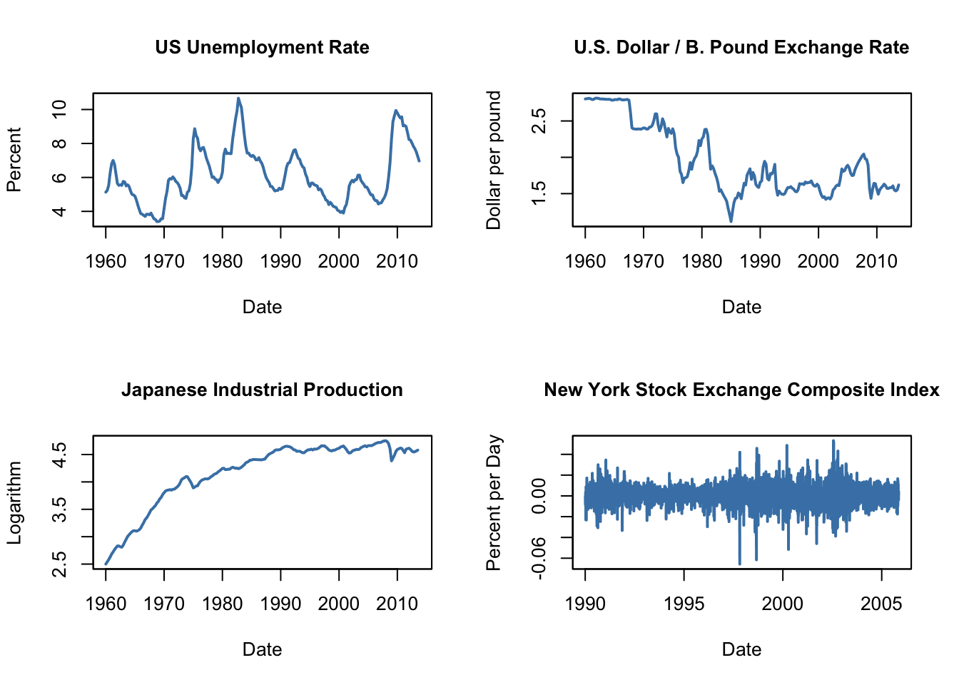
Any data recorded with some fixed interval of time is called time series data. This fixed interval can be hourly, daily, monthly, or yearly. e.g. hourly temp reading, daily changing fuel prices, monthly electricity bill, annual company profit report, etc. In time series data, time will always be an independent variable, and there can be one or many dependent variables.

Sales forecasting time series with shampoo sales for every month will look like this,

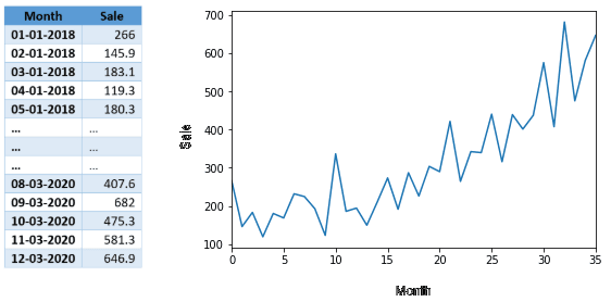
What is Time Series

In the above example, since there is only one variable dependent on time, it is called a univariate time series. If there are multiple dependent variables, then it is called a multivariate time series. The objective of time series data analysis is to understand how changes in time affect the dependent variables and accordingly predict values for future time intervals.

Components of Time Series Analysis

Time series data can be decomposed into four key components: trend, seasonality, cyclical, and irregularity.

Components of Time Series Analysis

Trend: A trend is a long-term pattern in the data that reflects the overall direction of the series. Trends can be upward, downward, or flat. For example, a company's stock prices might show an upward trend over several years, reflecting the overall growth of the company. We can use techniques like linear regression or moving averages to identify and model a trend.

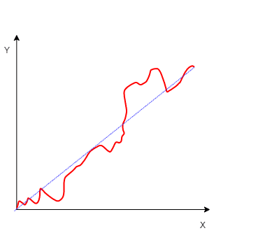
Trends

Seasonality: Seasonality refers to patterns in the data that repeat at regular intervals. For example, sales of winter coats might increase every year in the fall and winter months, reflecting seasonal demand. We can use techniques like seasonal decomposition or Fourier analysis to identify and model seasonality.

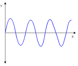
Seasonal patterns

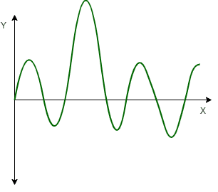
Cyclical: Cyclical patterns are similar to trends but are not fixed like seasonality. Instead, cyclical patterns occur when data experience a rise and fall that is not of a fixed frequency, like the business cycle in economics. We can use techniques like spectral or wavelet analysis to identify and model cyclical patterns.

Cyclical Patterns

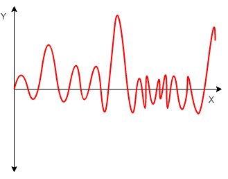
Irregularity: Irregularity, or noise, refers to the unpredictable fluctuations in the data that are not explained by trends, seasonality, or cyclical patterns. Randomness is important because it can affect the accuracy of predictions and models. We can use techniques like residual analysis or time series forecasting models to identify and model irregularity.

Irregularity

Example:  Let's say we are analyzing the monthly sales data of a clothing store. By plotting the data over time, we notice an upward trend in sales over several years. To model this trend, we can use linear regression to fit a straight line to the data. However, we also notice that sales of winter clothing increase during the fall and winter months, indicating seasonality. To model this seasonality, we can use seasonal decomposition to separate the data into its seasonal and non-seasonal components.

Additionally, we observe fluctuations that do not repeat at regular intervals, such as changes in fashion trends, representing the cyclical component. We can use techniques like spectral or wavelet analysis to model this cyclical pattern.

Data Types and Limitations

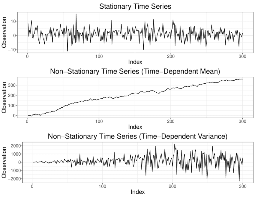
There are two main types of time series data: stationary and non-stationary.

Stationary time series data:

A stationary time series data is one where the statistical properties of the series, such as its mean, variance, and covariance, are constant over time. This means that the mean value of the data remains constant during the analysis, and the variance remains constant with respect to the time frame. Additionally, the covariance, which measures the relationship between two variables, remains constant over time. In other words, the data does not have any trend, seasonality, cyclical, or irregularity component.

Non-stationary time series data:

It is one where the statistical properties of the series change over time. This can occur when the mean, variance, or covariance changes with respect to time. Non-stationary data can have trend, seasonality, cyclical, and irregularity components and can be more challenging to analyze than stationary data.

Identifying whether a dataset is stationary or non-stationary is a crucial step in time series analysis, as it determines the appropriate modeling techniques to use. For example, if the data is non-stationary, it may be necessary first to transform the data to make it stationary before applying any analysis techniques.

Data Types and Limitations

Limitations of Time Series Analysis

• Missing values are not supported by TSA, similar to other models.
• The data points must have a linear relationship for proper analysis.
• Data transformations are mandatory, which can be expensive.
• TSA models typically work best on univariate data and may not perform as well with multivariate datasets.
• TSA assumes that the observations are equally spaced in time, which may not always be true in real-world scenarios.
• Time series analysis is sensitive to outliers, and the presence of outliers in the data can significantly affect the results of the analysis.

Time Series Analysis

Time series analysis involves the study of patterns in data over time. Let us go through a brief overview of various techniques and tests used for time series analysis.

Decomposition of Time Series:

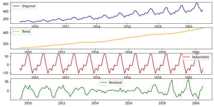
Decomposition of time series refers to the process of breaking down a time series into its individual components, namely trend, seasonality, cyclical, and irregularity. This technique is used to understand and analyze the underlying patterns and structures in the data.

Decomposition of time series can be done using various techniques, such as moving averages, exponential smoothing, and regression analysis. Once the individual components are identified, they can be modeled and analyzed separately to gain insights into the behavior and patterns of the time series data.

Decomposition of Time series

Stationarity:

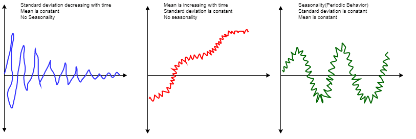
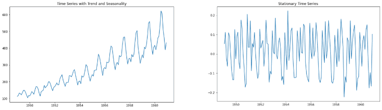
Stationary Data: In time series analysis, it is important to work with stationary data to make accurate forecasts and identify patterns. Stationary time series data is one where the statistical values, such as the mean and standard deviation, are constant over time. This means that the data does not have any trend or seasonality, and the statistical properties of the data should not be a function of time. In other words, the data should have a constant mean, variance, and covariance. By removing trends and seasonality from the time series data, it can be transformed into a stationary series, which is easier to analyze and model.

Stationarity

Test for Stationarity:

One simple way to identify stationarity is by visually examining the plot of the time series data for any noticeable trend or seasonality. However, for real-world data, more advanced techniques like rolling statistics and the Augmented Dickey-Fuller test can be utilized to determine the stationarity of the data.

Rolling Statistics:

Rolling statistics is a time series analysis technique that involves calculating statistical metrics, such as the mean and standard deviation, within a defined window size as it moves across the series. The size of the window is typically set based on the frequency of the data, such as daily or monthly.

For stationary time series data, the mean and standard deviation should remain constant over time, which can be verified by using rolling statistics. If there are no significant changes in the calculated mean and standard deviation values within the defined window size, then the data is likely to be stationary.

Augmented Dickey-Fuller (ADF) Test:

The Augmented Dickey-Fuller (ADF) test is a statistical test used to determine whether a time series is stationary or non-stationary. The test is based on the idea of regression, where the dependent variable is the time series itself, and the independent variable is a lagged version of the series.

The null hypothesis of the ADF test is that the time series is non-stationary.

ADF test will return 'p-value' and 'Test Statistics' output values.

• P-Value:

Null Hypothesis (H0): Series is non-stationary

Alternate Hypothesis (HA): Series is stationary

• p-value >0.05 Fail to reject (H0)

• p-value <= 0.05 Accept (H1)

• Test statistics: More negative this value is, the more likely we have stationary series. Also, this value should be smaller than critical values(1%, 5%, 10%). For e.g., if the test statistic is smaller than the 5% critical values, then we can say with 95% confidence that this is a stationary series.

The ADF test is a widely used technique in time series analysis and is particularly useful when working with real-world data that may have a trend or seasonality components. It helps to ensure that the time series is stationary before applying any further analysis or modeling techniques.

Converting Non-Stationary Data to Stationary Data

To make time series data stationary, it is important to account for its characteristics, such as trend and seasonality. This can be achieved by making the mean and variance of the time series constant. Below are some techniques that are commonly used to make non-stationary data stationary:

Differencing:

The differencing technique helps in removing trend and seasonality from time series data. It is performed by subtracting the previous observation from the current observation. The differenced data will contain one less data point than the original data. Differencing reduces the number of observations and stabilizes the mean of a time series.

After performing differencing, it is recommended to plot the data to visualize the change. If there is not sufficient improvement, we can perform second or third-order differencing.

Transformation:

Transformation Another technique to stabilize the variance across time is to apply a power transformation to the time series. Log, square root, and cube root are the most commonly used transformation techniques. Depending on the growth of the time series, we can choose the appropriate transformation method. For example, a time series with a quadratic growth trend can be made linear by taking the square root. If differencing doesn't work, we may use one of the above transformation techniques to remove the variation from the series.

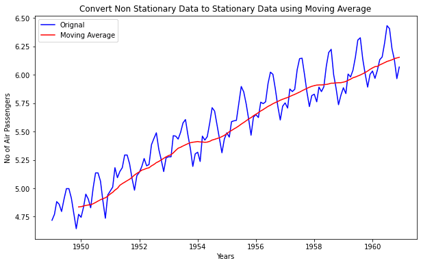
Moving Average:

Moving average is a time series technique that involves creating a new series by taking averages of data points from the original series. To calculate the average, two or more raw data points can be used, which is also known as the 'window width'. The averages are calculated from the start to the end for each set of w consecutive values, giving it the name moving averages. This technique can also be utilized for time series forecasting.

Moving Average

Weighted Moving Averages(WMA):

Weighted Moving Averages (WMA) is a method used in technical analysis to give more importance to recent data points while assigning less weight to data points that are far in the past. To calculate WMA, each value in the data set is multiplied by a pre-determined weight, and the resulting products are summed up. There are several ways to assign weights, and one of the commonly used methods is Exponential Weighted Moving Average, where weights are assigned to past values based on a decay factor.

Centered Moving Averages (CMA):

A centered moving average calculates the value of the moving average at time t by centering the window around time t and computing the average of the w values within the window. For instance, a centered moving average with a window of 3 is calculated as follows:

Centered Moving Averages

CMA is a useful technique for visualizing time series data.

Trailing Moving Averages (TMA):

In contrast to centered moving averages, trailing moving averages calculate the average of the last w values rather than averaging over a window centered around a time period of interest. For example, a trailing moving average with a window of 3 would be calculated as:

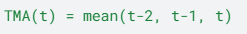
TMA

TMA is useful for forecasting.

Correlation

The most significant aspect of values in a time series is their dependence on previous values. We can determine the correlation between time series observations and previous time steps, known as lags. Because the correlation of time series observations is calculated with the values of the same series at previous times, this is referred to as autocorrelation or serial correlation.

To illustrate this point, let's consider the example of fish prices,

where

• P(t) represents the fish price of today,
• P(t-1) represents the fish price of the previous month, and
• P(t-2) represents the fish price of the month before that.

A time series of fish prices can be represented as P(t-n), ... P(t-3), P(t-2), P(t-1), P(t). By analyzing fish prices over the past few months, we can predict the fish price for today.

All past and future data points are interrelated in time series, and ACF and PACF functions assist in determining the correlation between them.

Auto Correlation Function (ACF)

• ACF determines the correlation between points based on the number of time steps separating them.
• For example, in the fish price example, we can determine the correlation between the current month's fish price P(t) and the fish price two months ago P(t-2).
• It is necessary to note that the fish price of two months ago can directly or indirectly affect today's fish price, possibly through last month's price P(t-1). ACF considers both direct and indirect effects between points while determining correlation.

Partial Auto Correlation Function (PACF)

• In contrast to ACF, PACF considers only direct effects between points while determining the correlation.
• For example, in the fish price example, PACF determines the correlation between the current month's fish price P(t) and the fish price two months ago P(t-2) by considering only P(t) and P(t-2) and ignoring P(t-1).

Time Series Forecasting

Time series forecasting involves making future predictions based on the analysis of past data points. The following steps are generally followed during time series forecasting:

1. Analyze the time series characteristics, such as trends and seasonality, to gain a better understanding of the data.
2. Determine the best method to make the time series stationary through data analysis.
3. Record the transformation steps used to make the time series stationary and ensure that the data can be transformed back to its original scale.
4. Choose an appropriate model for time series forecasting based on the data analysis.
5. Assess the model's performance using metrics such as a residual sum of squares (RSS), using the entire data set for prediction.
6. Transform the array of predictions back to the original scale to obtain the actual forecasted values.
7. Finally, conduct future forecasting to obtain forecasted values in the original scale.

Models Used For Time Series Forecasting

• Autoregression (AR)
• Moving Average (MA)
• Autoregressive Moving Average (ARMA)
• Autoregressive Integrated Moving Average (ARIMA)
• Seasonal Autoregressive Integrated Moving-Average (SARIMA)
• Seasonal Autoregressive Integrated Moving-Average with Exogenous Regressors (SARIMAX)
• Vector Autoregression (VAR)
• Vector Autoregression Moving-Average (VARMA)
• Vector Autoregression Moving-Average with Exogenous Regressors (VARMAX)
• Simple Exponential Smoothing (SES)
• Holt Winter’s Exponential Smoothing (HWES)

Applications of Time Series Analysis

Here are a few real-world applications where time series analysis is used

1. Sales Forecasting: Predict future sales based on historical sales data to help businesses plan for inventory management and production schedules.
2. Stock Market Analysis: Analyzing historical stock prices and market trends to make investment decisions and predict future market movements.
3. Energy Demand Forecasting: Predicting future energy demand based on historical usage patterns to help energy providers manage their supply and distribution networks.
4. Traffic Flow Analysis: Analyzing historical traffic data to identify patterns and predict future traffic congestion, helping city planners and transportation authorities to optimize traffic flow.
5. Weather Forecasting: Analyzing historical weather data to predict future weather patterns, helping meteorologists to issue accurate weather forecasts.
6. Epidemiological Analysis: Analyzing historical disease outbreak data to predict future outbreaks, helping public health officials to take preventive measures.
7. Website Traffic Analysis: Analyzing historical website traffic data to identify patterns and predict future traffic, helping website owners to optimize their content and advertising strategies.
8. Social Media Analysis: Analyzing historical social media data to identify trends and predict future consumer behavior, helping businesses to tailor their marketing strategies.
9. Financial Risk Analysis: Analyzing historical financial data to identify risk factors and predict future financial risks, helping investors and financial institutions to make informed decisions.

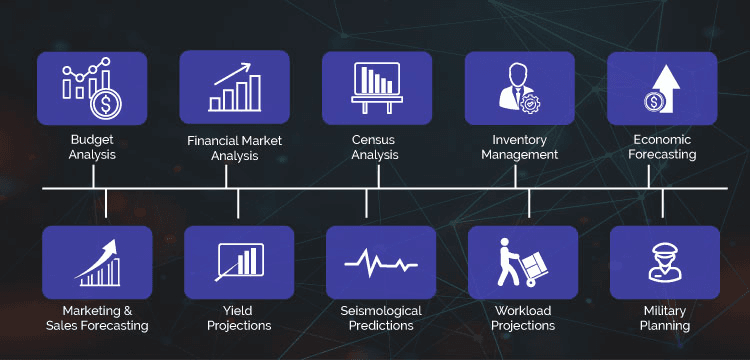
Applications of Time Series Analysis

Conclusion:

Time series analysis is a powerful statistical method for analyzing and forecasting time-dependent data. It can help identify patterns and trends in the data, understand the relationships between different variables, and predict future behavior. By using various techniques such as moving averages, autocorrelation, and regression analysis, time series analysis can provide valuable insights for decision-making in various fields such as finance, economics, engineering, and environmental science. However, it's important to note that time series analysis is not a panacea and requires careful consideration of the data and the assumptions underlying the models.