XGBoost In-depth Intuition

As the other algorithms take the independent features and try to predict the dependent one, same for Xgboost, but it doesn’t take the actual dependent feature, instead it creates its own feature, isn’t that amazing?

Let’s check how it works with the help of this table.

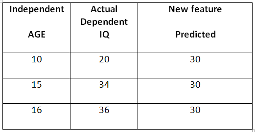
So, this is a simple example of predicting the IQ level with the help of age, but the column “**New feature (predicted)**” is the one which Xg-boost created by taking the average of all the IQ present in the table. As mentioned, it will take the new column and train itself, but this is not the main column/feature. Let’s have a look at this

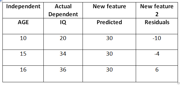
This is the new and final feature from which the training begins in Xg-boost. Now it will try to predict the residuals with the help of decision trees.

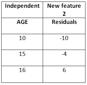
As we know the splitting criteria in decision trees, with the help of information gain. So the root node will be split if it shows the maximum information gain, and this tree will be the base learner or the weak learner and will predict the new values for residuals and which when added to the previous** “New feature (predicted)” **will give the new values of IQ, now again the same procedures go and Xg-boost learn from the mistakes of this base learner and will predict new values and so on until the loss or residuals are minimum, and we have our strong learner at the end. The advantage of this approach is that the new learners are being added to the model by learning and correcting the mistakes of previous learners.

Let’s have a look to practical example in python

• !pip install xgboost
• Import xgboost as xgb

Splitting and fitting the data

• from sklearn.model_selection import train_test_split
• X_train, X_test, Y_train, Y_test = train_test_split(X, y, test_size=0.2)

We need to change the format that Xg-boost can handle

• D_train = xgb.DMatrix(X_train, label=Y_train)
• D_test = xgb.DMatrix(X_test, label=Y_test)

we can define the parameters of our gradient boosting ensemble

• param = {
• ‘eta’: 0.3,
• ‘max_depth’: 3,
• ‘objective’: ‘multi:softprob’,
• ‘num_class’: 3}

steps = 10 # The number of training iterations

Training and testing

model = xgb.train(param, D_train, steps)

preds = model.predict(D_test)

Fighting with Overfitting

This is a very usual case in this algorithm because the algorithm is going through the data so many times, so it may learn the underlying logic very well, but we have a remedy for that, by using the hyper-parameter “Gamma”.

Minimum loss reduction required to make a further partition on a leaf node of the tree. The larger gamma is, the more conservative the algorithm will be.

Reference - https://xgboost.readthedocs.io/

Other parameters we can look into:- max_depth, and eta (the learning rate)

Special Notes –

We can use grid search for choosing the optimal hyper-parameters

Although it’s a boosting technique but it uses all the cores of our computer’s processor in a parallel manner, so we can also say this as a parallel technique but not directly, as the work is sequential.

References -

https://xgboost.readthedocs.io/

https://www.geeksforgeeks.org/xgboost-for-regression/