Joint Distributions, Covariance and Correlation

Joint distributions and covariance are essential concepts in probability theory and statistics. The joint distribution of random variables is the probability distribution of a set of random variables, whereas covariance measures the degree to which two random factors change together.

Joint Distributions

Joint distributions are probability distributions that describe the relationship between two or more random variables. A joint distribution specifies the probability of each possible combination of values for the random variables. The joint probability density function (PDF) for two continuous random variables X and Y is denoted as f(x, y), while for two discrete random variables X and Y, it is denoted as P(X = x, Y = y).

Example: Suppose we have two random variables X and Y that represent the number of heads and tails, respectively, in two coin flips. The joint distribution of X and Y can be represented as follows:

Example: Suppose we have two random variables X and Y that represent the number of heads and tails, respectively, in two coin flips. The joint distribution of X and Y can be represented as follows:

Marginal Distributions

Marginal distributions refer to the probability distributions of individual random variables obtained from a joint distribution. The marginal distribution of X is obtained by summing (in the discrete case) or integrating (in the continuous case) over all possible values of Y.

Example: Using the joint distribution from the previous example, the marginal distribution of X can be obtained as follows:

Conditional Distributions

Conditional distributions portray the probability distribution of one irregular variable given the esteem of another. The conditional conveyance of Y given X is indicated as P(Y | X) or f(Y | X), and is calculated by dividing the joint distribution of X and Y by the marginal distribution of X.

To find the conditional probability of X given Y, we need to use the formula:

P(X|Y) = P(X and Y) / P(Y)

Illustration:

Utilizing the joint dissemination from the past illustration, the conditional distribution of Y given X=1 can be gotten as follows:

Let's find the conditional probability of X = 1 given Y = 2:

P(X=1|Y=2) = P(X=1 and Y=2) / P(Y=2)

P(X=1 and Y=2) = 1/2 (from the table)

P(Y=2) = 1/4 + 1/2 + 1/4 = 1 (sum of probabilities in the Y=2 column)

Therefore,

P(X=1|Y=2) = (1/2) / 1 = 1/2

So the conditional probability of X=1 given Y=2 is 1/2.

Covariance and Correlation

Covariance measures the degree to which two random variables X and Y are linearly related. It is defined as the expected value of the product of the deviations of X and Y from their respective means:

cov(X,Y) = E[(X - E[X])(Y - E[Y])]

Correlation is a standardized version of covariance, and measures the degree of linear association between two variables X and Y:

corr(X,Y) = cov(X,Y) / (std(X) * std(Y))

Example:

To find the covariance and correlation between X and Y, we need to use the following formulas:

Cov(X,Y) = E[XY] - E[X]E[Y]

Corr(X,Y) = Cov(X,Y) / (SD(X) * SD(Y))

where E[XY] is the expected value of the product of X and Y, E[X] and E[Y] are the expected values of X and Y, SD(X) and SD(Y) are the standard deviations of X and Y, respectively.

Let's start by finding the expected values of X and Y:

E[X] = 0*(1/4) + 1*(1/2) + 2*(1/4) = 1

E[Y] = 0*(1/2) + 1*(1) + 2*(1/2) = 1

Next, let's find the expected value of XY:

E[XY] = 00(1/4) + 01(1/2) + 02(1/4)
                + 10(1/2) + 11(0) + 12(1/2)
                + 20(1/4) + 21(1/2) + 22(1/4)

= 0 + 0 + 0 + 0 + 0 + 1 + 0 + 2 + 1 = 4/2 = 2

Now, let's calculate the standard deviations of X and Y:

SD(X) = sqrt(E[X^2] - (E[X])^2)
            = sqrt(0*(1/4) + 1*(1/2) + 4*(1/4) - 1^2) = sqrt(1/4) = 1/2

SD(Y) = sqrt(E[Y^2] - (E[Y])^2)
            = sqrt(0*(1/2) + 1*(1) + 4*(1/2) - 1^2) = sqrt(3/2)

Now, we can calculate the covariance between X and Y:

Cov(X,Y) = E[XY] - E[X]E[Y]
                 = 2 - (1)*(1) = 1

Finally, we can calculate the correlation between X and Y:

Corr(X,Y) = Cov(X,Y) / (SD(X) * SD(Y))
                    = 1 / ((1/2) * sqrt(3/2)) = sqrt(8/3)

So the covariance between X and Y is 1 and the correlation between X and Y is approximately 1.63299.

Correlation

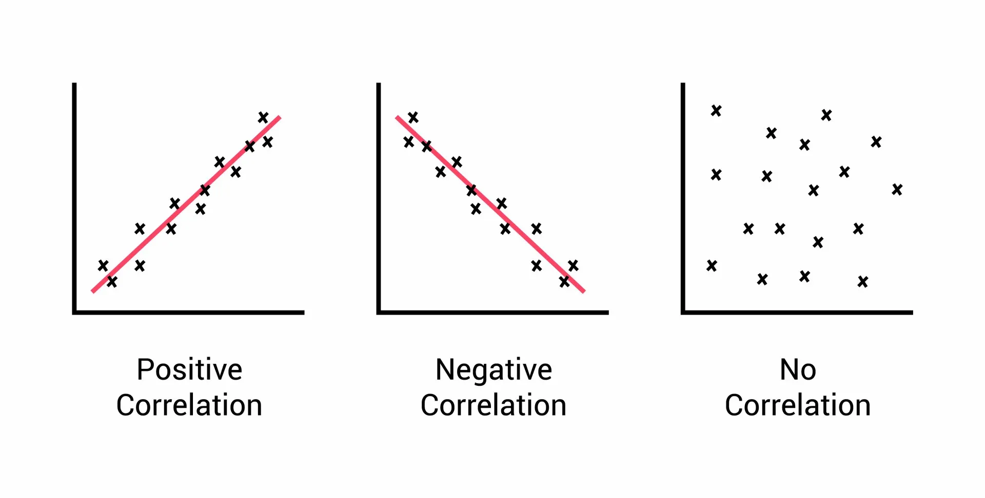
Correlation is a statistical measure used to determine the degree to which two variables are related to each other. Correlation can be either positive or negative, indicating the direction of the relationship between the variables. A positive correlation means that as one variable increases, the other variable also increases, while a negative correlation means that as one variable increases, the other variable decreases.

Types of Correlation and their ApplicationsTypes of Correlation and their Applications

There are three main types of correlation: positive correlation, negative correlation, and zero correlation.

Types of Correlation

Positive Correlation

Positive correlation occurs when the values of two variables increase or decrease together. For example, there is a positive correlation between the amount of exercise people do and their level of fitness. The more exercise people do, the fitter they are likely to be.

The formula for calculating the Pearson correlation coefficient for a positive correlation is:

r = (nΣxy - ΣxΣy) / sqrt[(nΣx^2 - (Σx)^2)(nΣy^2 - (Σy)^2)]

where:

• n is the number of data points
• Σxy is the sum of the products of each pair of corresponding x and y values
• Σx is the sum of all x values
• Σy is the sum of all y values
• Σx^2 is the sum of the squares of all x values
• Σy^2 is the sum of the squares of all y values

Negative Correlation

Negative correlation occurs when the values of two variables move in opposite directions. For example, there is a negative correlation between the amount of time people spend watching TV and their level of physical activity. The more time people spend watching TV, the less physically active they are likely to be.

The formula for calculating the Pearson correlation coefficient for a negative correlation is:

r = (nΣxy - ΣxΣy) / sqrt[(nΣx^2 - (Σx)^2)(nΣy^2 - (Σy)^2)]

Where:

• n is the number of data points
• Σxy is the sum of the products of each pair of corresponding data points (x and y)
• Σx is the sum of all the x values
• Σy is the sum of all the y values
• Σx^2 is the sum of the squared x values
• Σy^2 is the sum of the squared y values

Zero Correlation

Zero correlation occurs when there is no relationship between the two variables. For example, there is no correlation between the color of someone's eyes and their shoe size.

Multivariate Distributions

Multivariate distributions generalize joint distributions to more than two random variables.A multivariate distribution indicates the probability distribution of a set of random variables, where each arbitrary variable may have a different probability distribution. A few commonly utilized multivariate dispersions incorporate the multivariate ordinary dispersion, the multinomial distribution, and the multivariate t-distribution.

Illustration: Assume we have three arbitrary factors X, Y, and Z, where X and Y are ceaseless random variables and Z may be a discrete random variable. The joint distribution of X, Y, and Z can be spoken to as takes after:

f(x, y, z) = P(X = x, Y = y, Z = z)

Applications of Joint Distributions

Joint distributions and covariance have numerous applications in statistics, probability theory, and data analysis. They are used in fields such as finance, engineering, biology, and machine learning. Some applications of joint distributions include:

• Portfolio optimization: Joint distributions are used to model the relationship between the returns of different assets in a portfolio and optimize portfolio allocations.
• Signal processing: Joint distributions are used to model the joint probability distribution of signals and to estimate parameters such as signal power and correlation.
• Genetics: Joint distributions are used to model the joint probability distribution of genetic traits and to estimate heritability and gene expression levels.
• Machine learning: Joint distributions are used in various machine learning algorithms, such as Gaussian mixture models, hidden Markov models, and Bayesian networks, to model complex dependencies between variables.
• Bayesian inference: Joint distributions are utilized in Bayesian inference to upgrade earlier beliefs about model parameters based on watched information.
• Time series investigation: Joint distributions are utilized to demonstrate the joint probability distribution of time series data and to assess parameters such as autocorrelation and cross-correlation.

Conclusion

In conclusion, joint distributions, correlation and covariance are essential concepts in probability theory and insights that play a vital part in different applications. They permit us to show the connections between different random variables and measure the degree to which they shift together. From fund to genetics and machine learning, joint distributions and covariance are utilized broadly to analyze information, make forecasts, and educate decision-making.

Key Takeaways

1. Joint distributions are the probability distribution of a set of random variables.
2. Covariance measures the degree to which two random variables vary together.
3. The correlation coefficient is the standardized covariance between two random variables.
4. The joint distribution of two random variables can be visualized with a scatter plot.
5. Multivariate distributions can model the joint distribution of more than two random variables.
6. Joint distributions and covariance have numerous applications in finance, engineering, biology, machine learning, Bayesian inference, and time series analysis.
7. Correlation measures the strength and direction of the relationship between two variables

Quiz

1. What is the joint distribution of two random variables? 

A. The probability distribution of a single random variable 

B. The probability distribution of a set of random variables 

C. The distribution of the difference between two random variables 

D. The distribution of the sum of two random variables

Answer: B

2. What does covariance measure? 

A. The degree to which two random variables vary together 

B. The degree to which two random variables are independent 

C. The standard deviation of a single random variable 

D. The probability of observing two random variables together

Answer: A

3. Which of the following measures the strength of the linear relationship between two random variables? 

A. Variance 

B. Correlation coefficient 

C. Standard deviation 

D. Mean

Answer: B

4. What is the main application of joint distributions and covariance in finance? 

A. Estimating heritability and gene expression levels 

B. Modeling the joint probability distribution of signals 

C. Modeling the relationship between the returns of different assets in a portfolio 

D. Modeling the joint probability distribution of time series data

Answer: C

5. What is the correlation coefficient?

A) A measure of the strength and direction of the linear relationship between two variables. 

B) A measure of the strength and direction of the non-linear relationship between two variables. 

C) A measure of the probability that two variables are related. 

D) A measure of the magnitude of the difference between two variables.

Answer: A) A measure of the strength and direction of the linear relationship between two variables.

6. What is the range of possible values for the correlation coefficient?

A) -1 to 1 

B) 0 to 1 

C) -∞ to ∞ 

D) 0 to ∞

Answer: A) -1 to 1