Probability and Fundamental Principle of Counting

It is the branch of mathematics concerned with quantifying uncertainty and predicting the likelihood of events. It covers basic concepts such as events, outcomes, and sample spaces, as well as the probability of an event and its relationship to impossible and certain events. Additionally, the article introduces the counting principles and their application to probability calculations.

Introduction to Probability and Counting Principles

Probability is the branch of mathematics that deals with the study of random events. It allows us to quantify uncertainty and make predictions about the likelihood of certain events occurring. In this article, we will discuss the basic concepts of probability and the counting principles.

Basic Concepts in Probability

An event is a collection of outcomes. An outcome is the result of an experiment. A sample space is the set of all possible outcomes of an experiment. For example, if we toss a coin, the sample space consists of two possible outcomes: heads and tails. If we roll a die, the sample space consists of six possible outcomes: 1, 2, 3, 4, 5, or 6.

The probability of an event is a number between 0 and 1, inclusive, that represents the likelihood of the event occurring. If an event is impossible, its probability is 0. If an event is certain, its probability is 1. For example, the probability of rolling a 7 on a standard die is 0, and the probability of rolling a number less than 7 on a standard die is 1.

Types of Probability

There are three types of probability: classical, empirical, and subjective probability.

1. Classical probability is based on theoretical analysis and assumes that all outcomes in a sample space are equally likely to occur. The probability of an event A is the number of outcomes that favor A divided by the total number of outcomes in the sample space. For example, the probability of rolling a 1 on a standard die is 1/6, and the probability of rolling an even number on a standard die is 3/6 = 1/2.
2. Empirical probability is based on experimental data and involves observing the frequency of an event occurring over many trials. The probability of an event A is the number of times A occurs divided by the total number of trials. For example, if we roll a die 100 times and record the number of times each number appears, we can estimate the probability of rolling each number based on the frequency of occurrence.
3. Subjective probability is based on personal judgments and opinions and is often used in situations where there is no empirical or theoretical basis for calculating probabilities. For example, a weather forecaster may estimate the probability of rain based on his or her experience and knowledge of the weather patterns in the area.

Counting Principles

The counting principle is a set of rules that can be used to count the number of possible outcomes in a sample space.

1. Permutations

A permutation is a arrangement of objects in a particular order. The number of permutations of n objects taken r at a time is denoted by P(n, r) and is given by:

P(n, r) = n! / (n - r)!

where n! represents the factorial of n, which is the product of all positive integers up to and including n.

For example, the number of ways to arrange three letters out of the five letters A, B, C, D, and E is

P(5, 3) = 5! / (5 - 3)! = 60

2. Combinations

A combination is a selection of objects in which order is not important. The number of combinations of n objects taken r at a time is denoted by C(n, r) and is given by:

C(n, r) = n! / (r! * (n - r)!)

For example, the number of ways to choose two letters out of the five letters A, B, C, D, and E is

C(5, 2) = 5! / (2! * (5 - 2)!) = 10

3. Binomial Coefficient

The binomial coefficient is a number that represents the number of ways to choose r objects out of n objects. The binomial coefficient is denoted by C(n, r) and is given by:

C(n, r) = n! / (r! * (n - r)!)

The binomial coefficient is often used in the binomial probability distribution, which is used to model the probability of a certain number of successes in a fixed number of trials, where each trial has only two possible outcomes.

For example, if we flip a coin 3 times, the probability of getting exactly 2 heads is given by:

P(X = 2) = C(3, 2) * (1/2)^2 * (1/2)^1 = 3/8

where X is the number of heads.

Probability Distributions

A probability distribution is a function that describes the likelihood of different outcomes in a random experiment. There are two types of probability distributions:

1. Discrete probability distributions
2. Continuous probability distributions.

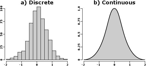
Probability Distributions

A discrete probability distribution is a probability distribution where the random variable can take on a finite number of values. Examples of discrete probability distributions include the binomial distribution, Poisson distribution, and geometric distribution.

1. Binomial Distribution

The binomial distribution is a discrete probability distribution that models the probability of a certain number of successes in a fixed number of independent trials, where each trial has only two possible outcomes. The binomial distribution is characterized by two parameters: the number of trials n and the probability of success p.

The probability mass function (PMF) of the binomial distribution is given by:

P(X=k) = C(n,k) * p^k * (1-p)^(n-k)

where X is the random variable that represents the number of successes, k is the number of successes, C(n,k) is the binomial coefficient, and p is the probability of success.

For example, if we flip a coin 10 times and want to know the probability of getting exactly 5 heads, we can use the binomial distribution with n=10 and p=0.5:

P(X=5) = C(10,5) * 0.5^5 * (1-0.5)^(10-5) = 0.2461

2. Poisson Distribution

The Poisson distribution is a discrete probability distribution that models the probability of a certain number of events occurring in a fixed interval of time or space, given that the events occur independently of each other and at a constant rate. The Poisson distribution is characterized by one parameter: the mean number of events λ.

The probability mass function (PMF) of the Poisson distribution is given by:

P(X=k) = e^(-λ) * λ^k / k!

where X is the random variable that represents the number of events, k is the number of events, e is the mathematical constant approximately equal to 2.71828, and k! is the factorial of k.

For example, if we want to know the probability of observing 3 accidents per day on a certain road, given that the average number of accidents per day is 2, we can use the Poisson distribution with λ=2:

P(X=3) = e^(-2) * 2^3 / 3! = 0.1804

3. Geometric Distribution

The geometric distribution is a discrete probability distribution that models the probability of the number of trials needed to obtain the first success in a sequence of independent trials, where each trial has only two possible outcomes. The geometric distribution is characterized by one parameter: the probability of success p.

The probability mass function (PMF) of the geometric distribution is given by:

The probability mass function (PMF) of the geometric distribution is given by:

P(X=k) = (1-p)^(k-1) * p

where X is the random variable that represents the number of trials needed to obtain the first success, k is the number of trials needed, and p is the probability of success.

For example, if we want to know the probability of flipping a coin 4 times before getting the first head, we can use the geometric distribution with p=0.5:

For example, on the off chance that we want to know the probability of flipping a coin 4 times some time recently getting the first head, we will utilize the geometric dissemination with p=0.5:

P(X=4) = (1-0.5)^(4-1) * 0.5 = 0.0625

Continuous Probability Distributions

A continuous probability distribution is a probability distribution where the random variable can take on any value within a certain range. Examples of continuous probability distributions include the normal distribution, exponential distribution

1. Exponential Distribution

The exponential distribution is a continuous probability distribution that models the probability of the time between two consecutive events in a Poisson process. A Poisson process is a process where events occur randomly and independently of each other at a constant rate. The exponential distribution is characterized by one parameter: the rate parameter λ.

The probability density function (PDF) of the exponential distribution is given by:

f(x) = λe^(-λx)

where x is the time between two consecutive events.

For example, if we need to know the probability of holding up more than 5 minutes for the another bus, given that the buses arrive at a rate of 2 buses per hour, able to use the exponential dispersion with λ=1/30 (since there are 60 minutes in an hour):

P(X>5) = ∫[5, ∞] λe^(-λx) dx = e^(-λx)|[5, ∞] = e^(-λ*5) = 0.0821

2. Normal Distribution

The normal distribution, also known as the Gaussian distribution, is a continuous probability distribution that is commonly used to model real-world phenomena such as height, weight, and IQ scores. The normal distribution is characterized by two parameters: the mean μ and the standard deviation σ.

The probability density function (PDF) of the normal distribution is given by:

f(x) = (1/σ√(2π)) * e^(-((x-μ)^2)/(2σ^2))

where x is the variable of interest.

For example, if we want to know the probability of a person having a height between 170 cm and 180 cm, given that the population has a mean height of 175 cm and a standard deviation of 5 cm, we can use the normal distribution:

P(170 ≤ X ≤ 180) = ∫[170, 180] (1/5√(2π)) * e^(-((x-175)^2)/(2*5^2)) dx 
= 0.1359

Bayes' Theorem

Bayes' theorem is a mathematical formula that describes the probability of an event, based on prior knowledge of conditions that might be related to the event. It is named after Reverend Thomas Bayes, an 18th-century British statistician.

Bayes' theorem can be written as:

P(A|B) = P(B|A) * P(A) / P(B)

where P(A|B) is the probability of A given that B is true, P(B|A) is the probability of B given that A is true, P(A) is the prior probability of A, and P(B) is the prior probability of B.

For example, if we want to know the probability of a person having a disease, given that they test positive for the disease, we can use Bayes' theorem:

P(Disease|Positive) = P(Positive|Disease) * P(Disease) / P(Positive)

where P(Disease|Positive) is the probability of having the disease given a positive test result, P(Positive|Disease) is the probability of testing positive given the disease, P(Disease) is the prior probability of having the disease, and P(Positive) is the prior probability of testing positive.

Applications of Probability Theory

Probability theory has many applications in real-life scenarios, such as:

1. Risk management: Probability theory is used to calculate the risk of certain events happening and to develop strategies to mitigate or manage those risks.
2. Finance: Probability theory is used to model and predict the behavior of financial markets and to value financial instruments such as options and derivatives.
3. Insurance: Probability theory is used to calculate the likelihood of certain events, such as accidents or natural disasters, and to determine appropriate premiums for insurance policies.
4. Medical research: Probability theory is used in clinical trials to determine the efficacy of new drugs and treatments, and to assess the probability of adverse events.
5. Sports: Probability theory is used to predict the outcomes of sporting events and to develop betting strategies.
6. Weather forecasting: Probability theory is used to model the behavior of the atmosphere and to predict weather patterns.

Common Misconceptions about Probability

There are several common misconceptions about probability, and including

1. The law of large numbers guarantees that small sample sizes will be representative of the population: While the law of large numbers does state that the average of a large number of independent samples will converge to the true population mean, it does not guarantee that small sample sizes will be representative of the population.
2. The outcomes of independent events are not influenced by previous events: While this is true in theory, in practice, events may be dependent due to hidden factors or feedback loops.
3. The probability of an event occurring is always between 0 and 1: While this is true in many cases, there are situations where the probability of an event may be negative or greater than 1.
4. The probability of an event occurring is the same as the frequency of that event occurring: While the frequency of an event may provide some indication of its probability, it is not always a reliable indicator.

Conclusion

Probability theory is a fundamental branch of mathematics that has many applications in real-life scenarios. It provides a framework for analyzing and predicting the likelihood of events, and is essential for risk management, finance, insurance, medical research, sports, weather forecasting, and many other fields. By understanding the basic principles of probability theory and avoiding common misconceptions, we can make more informed decisions and better navigate the uncertainties of the world around us.

Key Takeaways

1. Probability theory is a branch of mathematics that deals with the analysis and prediction of the likelihood of events.
2. There are two types of probability distributions: discrete and continuous.
3. Bayes' theorem is a mathematical formula that allows us to update our beliefs about the probability of an event based on new information.
4. Probability theory has many real-life applications, including finance, insurance, medical research, sports, and weather forecasting.
5. There are several common misconceptions about probability, including the belief that small sample sizes are always representative of the population, and that the probability of an event is always between 0 and 1.
6. By understanding the basic principles of probability theory, we can make more informed decisions and better navigate the uncertainties of the world around us.

Quiz

1. What are the two types of probability distributions? 

a) Independent and dependent 

b) Linear and nonlinear 

c) Discrete and continuous 

d) Normal and exponential

Answer: c) Discrete and continuous

2. What is Bayes' theorem used for? 

a) Calculating the average of a large number of independent samples 

b) Updating our beliefs about the probability of an event based on new information 

c) Modeling the behavior of the atmosphere and predicting weather patterns 

d) Predicting the outcomes of sporting events and developing betting strategies

Answer: b) Updating our beliefs about the probability of an event based on new information

3. Which of the following is NOT a real-life application of probability theory? 

a) Risk management 

b) Medical research 

c) Social media marketing 

d) Weather forecasting

Answer: c) Social media marketing

4. What is a common misconception about probability? 

a) Small sample sizes are always representative of the population. 

b) The outcomes of independent events are always influenced by previous events. 

c) The likelihood of an occasion is always between and 1. 

d) The likelihood of an occasion happening is always the same as the recurrence of that occasion happening.

Answer: b) The outcomes of independent events are always influenced by previous events.