Decision Tree in Machine Learning

Decision Trees are supervised learning algorithms used for classification and regression problems. They work by creating a model that predicts the value of a target variable based on several input variables. The model is a tree-like structure, with each internal node representing a "test" on an attribute, each branch representing the outcome of the test, and each leaf node representing a class label.

What is Decision Tree in Machine Learning?

An example of how decision trees are used in industry is in the banking sector. Banks use decision trees to help them determine which loan applicants are most likely to be responsible borrowers. They can use the applicant’s data, such as income, job history, credit score, and other factors, to create a decision tree that will help them determine which applicants are most likely to pay back the loan. The decision tree can then be used to make decisions about loan applications and help the bank decide which applicants should receive the loan.

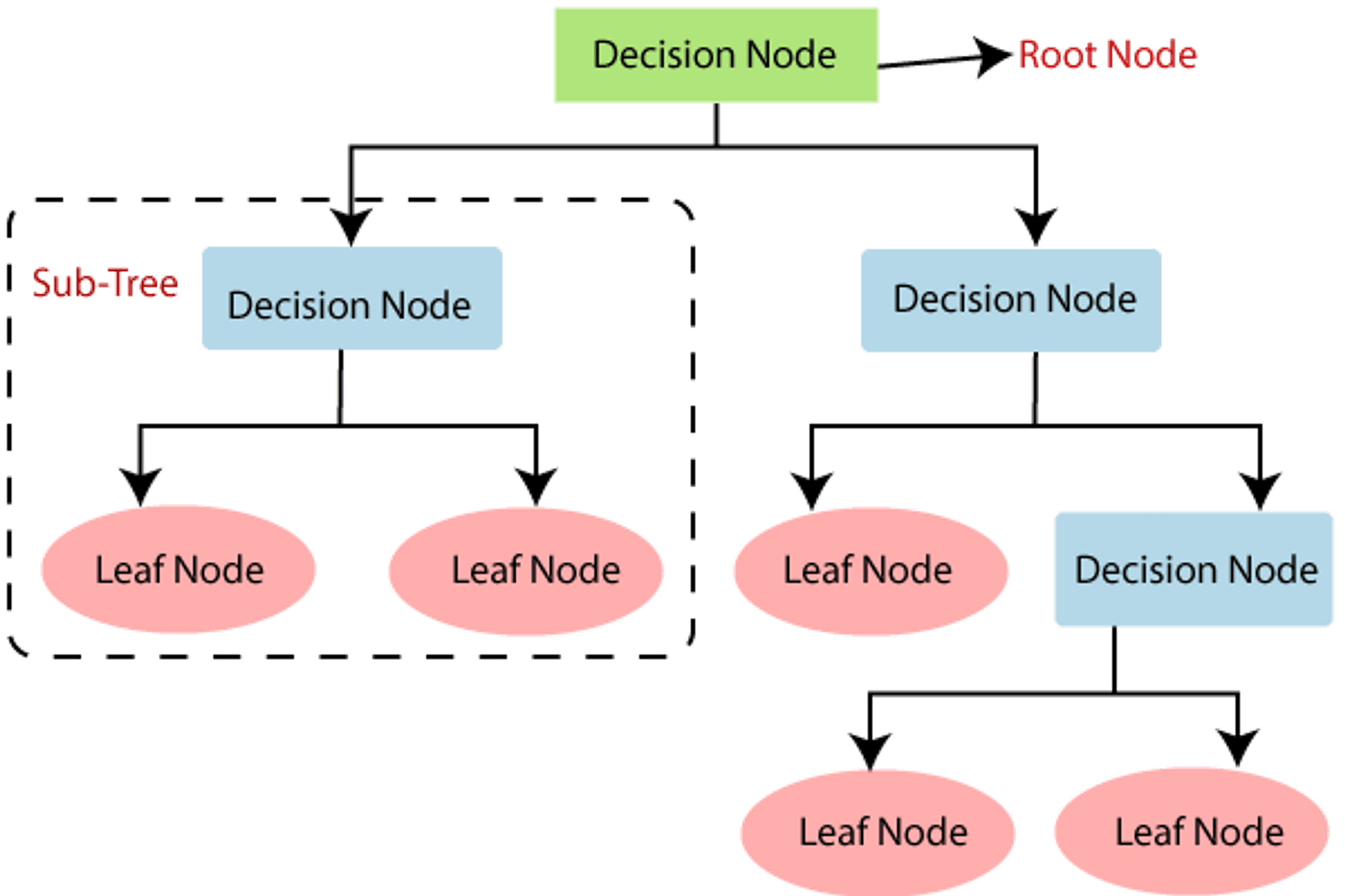
Decision Tree is a Supervised learning technique used for Classification and Regression problems. It consists of Decision Nodes and Leaf Nodes, where Decision Nodes make decisions based on given features and Leaf Nodes give the output of these decisions. It is a graphical representation for getting all the possible solutions to a problem/decision based on conditions. It uses the CART algorithm (Classification and Regression Tree algorithm) to build the tree. It starts with the root node and splits into subtrees based on the answer to questions posed.

Tree Construction

In a decision tree, the algorithm begins at the root node and works its way up to predict the class of a given dataset. This algorithm checks the values of the root property with the values of the record (actual dataset) attribute and then follows the branch and jumps to the next node depending on the comparison.

The decision tree algorithm in machine learning checks the attribute value with the other sub-nodes and moves on to the next node. It repeats the procedure until it reaches the tree's leaf node. The following algorithm will help you better understand the entire process:

Step 1: Begin the tree with the root node S, which includes the whole dataset. 

Step 2: Using the Attribute Selection Measure, find the best attribute in the dataset. 

Step 3: Subdivide the S into subsets containing potential values for the best qualities. 

Step 4: Create the decision tree node with the best attribute. 

Step 5: Create new decision trees recursively using the subsets of the dataset obtained in step3. Continue this procedure until you reach a point where you can no longer categorize the nodes and refer to the last node as a leaf node.

Example

Assume an applicant receives a job offer and must decide whether to take it or decline it. Hence, in order to address this problem, the decision tree begins at the root node (Salary attribute by ASM). Based on the labels, the root node divides further into the next decision node (distance from the workplace) and one leaf node. The following decision node is further subdivided into one decision node (Cab facility) and one leaf node. After that, the decision node divides into two leaf nodes (Accepted offers and Declined offer). Consider the diagram below: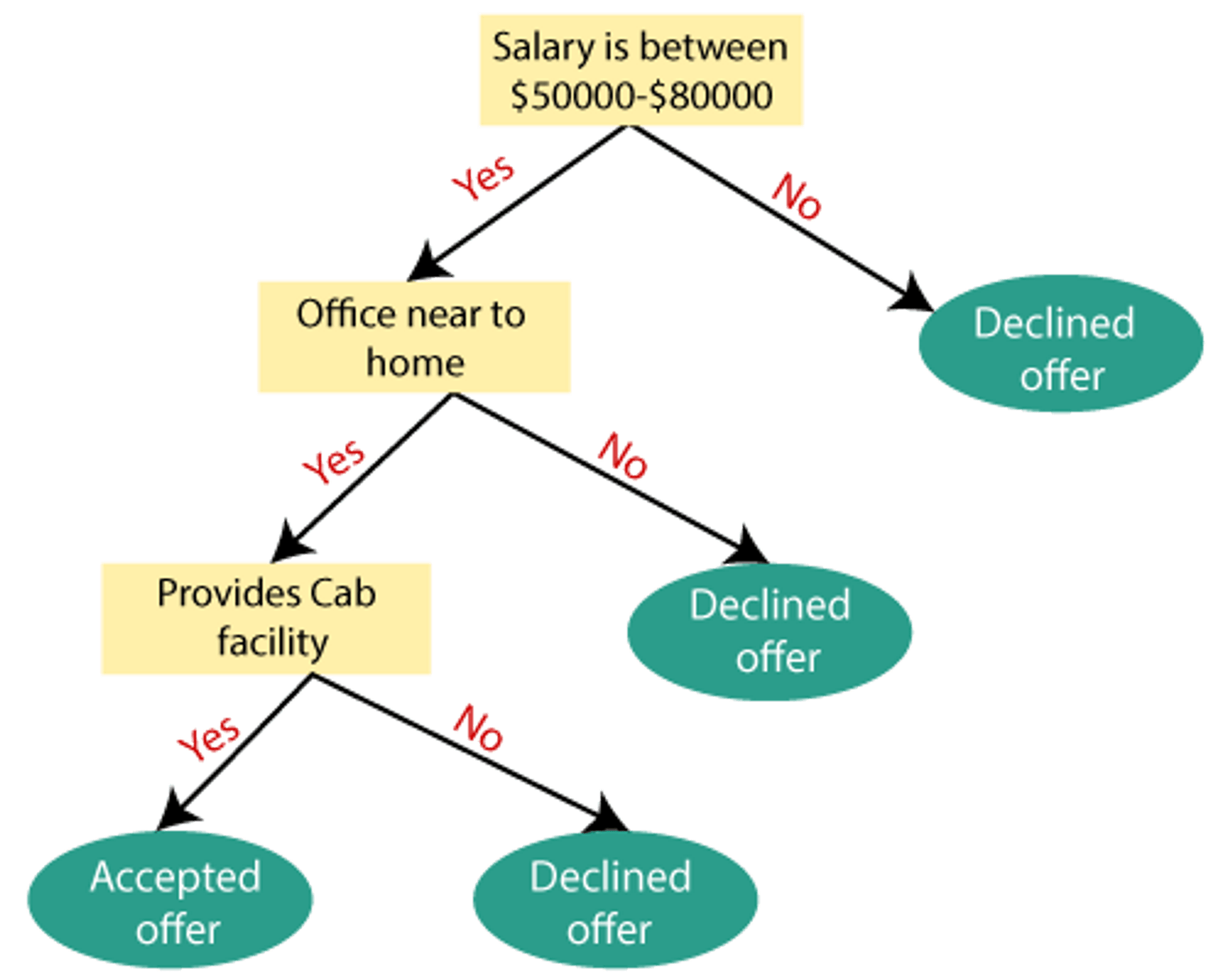

Attribute Selection Measures

The biggest challenge that emerges while developing a Decision tree is how to choose the optimal attribute for the root node and sub-nodes. To tackle such challenges, a technique known as Attribute selection measure, or ASM, is used. We can simply determine the best characteristic for the tree's nodes using this measurement. ASM is commonly performed using two techniques:

1. Information Gain

2. Gini index

Information Gain

Information gain is the assessment of changes in entropy following attribute-based segmentation of a dataset. It computes the amount of information a feature offers about a class. We divided the node and build the decision tree based on the importance of information obtained. A decision tree algorithm will always try to maximise the value of information gain, and the node/attribute with the most information gain will be split first. It may be computed using the formula below:

Information Gain= Entropy(S)- [(Weighted Avg) * Entropy(each feature)

Entropy: Entropy is a metric to measure the impurity in a given attribute. It specifies randomness in data. Entropy can be calculated as:

Entropy(s)= -P(yes)log2 P(yes)- P(no) log2 P(no)

Where,

• S= Total number of samples
• P(yes)= probability of yes
• P(no)= probability of no

Gini Index

The Gini index is a measure of impurity or purity utilised in the CART (Classification and Regression Tree) technique for generating a decision tree. A low Gini index attribute should be favoured over a high Gini index attribute. It only generates binary splits, whereas the CART method generates binary splits using the Gini index. The Gini index may be computed using the formula below:

Gini Index= 1- ∑jPj2

Examples

To Find Information Gain

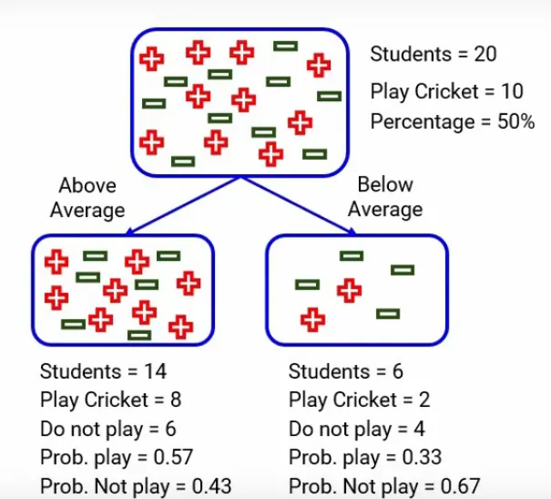
Let’s say we have a sample of 30 students with three variables Gender (Boy/Girl), Class(IX/X) and Height (5 to 6 ft). 15 out of these 30 play cricket in leisure time. Now, I want to create a model to predict who will play cricket during leisure period? In this problem, we need to segregate students who play cricket in their leisure time based on highly significant input variable among all three.

This is where decision tree helps, it will segregate the students based on all values of three variable and identify the variable, which creates the best homogeneous sets of students (which are heterogeneous to each other). In the snapshot below, you can see that variable Gender is able to identify best homogeneous sets compared to the other two variables.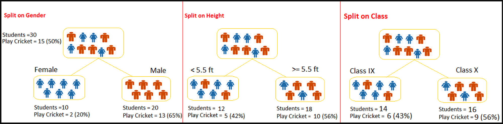

Now we want to segregate the students based on target variable ( playing cricket or not ). In the snapshot below, we split the population using two input variables Gender and Class. Now, I want to identify which split is producing more homogeneous sub-nodes using Information Gain.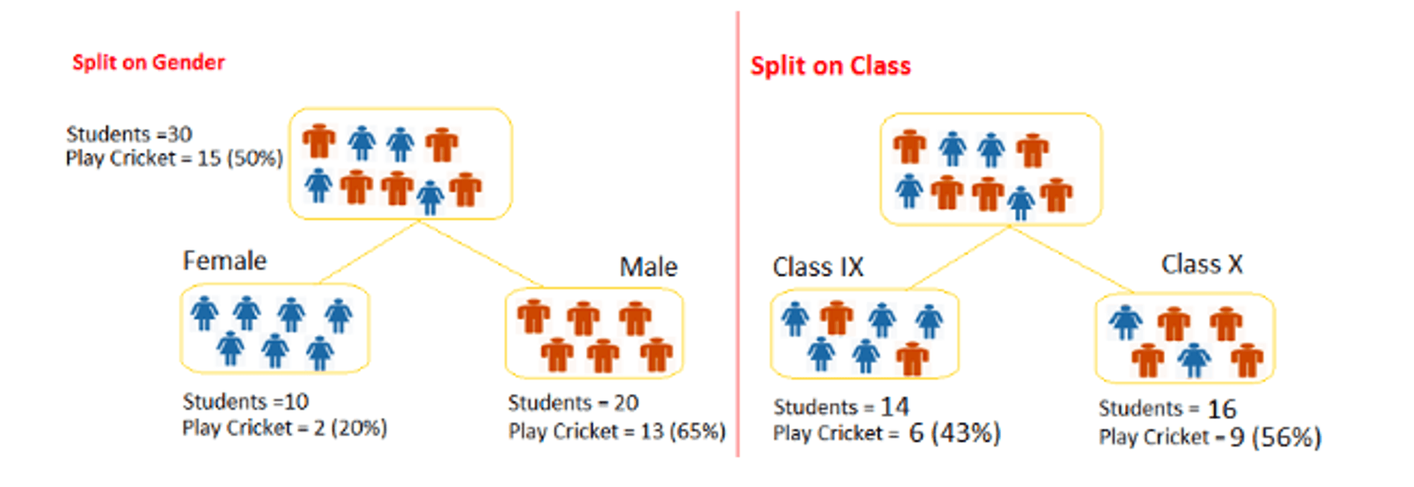

Entropy for parent node = - (15/30) log(15/30) – (15/30) log(15/30) = 1.

Here 1 shows that it is a impure node.

• Split on Gender:

Entropy for Female node = -(2/10) log(2/10) – (8/10) log(8/10) = 0.72 and for male node, -(13/20) log(13/20) – (7/20) log(7/20) = 0.93
Entropy for split Gender = Weighted entropy of sub-nodes = (10/30)*0.72 + (20/30)*0.93 = 0.86
Information Gain for split Gender = Entropy before split - Entropy after split = 1 - 0.86 = 0.14

• Split on Class:

Entropy for Class IX node, -(6/14) log(6/14) – (8/14) log(8/14) = 0.99 and for Class X node, -(9/16) log(9/16) – (7/16) log(7/16) = 0.99.
Entropy for split Class = (14/30)*0.99 + (16/30)*0.99 = 0.99

Information Gain for split Class = Entropy before split - Entropy after split = 1 - 0.99 = 0.01

Decision:

Above, we can see that Information Gain for split on Gender is the highest among all, so the tree will split on Gender.

To Find the Gini Index

Let’s use Gini method to identify best split for student example.

• Split on Gender:

Calculate, Gini for sub-node Female = (0.2)(0.2)+(0.8)(0.8)=0.68
Gini for sub-node Male = (0.65)(0.65)+(0.35)(0.35)=0.55
Calculate weighted Gini for Split Gender = (10/30)*0.68+(20/30)*0.55 = 0.59

• Similar for Split on Class:

Gini for sub-node Class IX = (0.43)(0.43)+(0.57)(0.57)=0.51
Gini for sub-node Class X = (0.56)(0.56)+(0.44)(0.44)=0.51
Calculate weighted Gini for Split Class = (14/30)*0.51+(16/30)*0.51 = 0.51

Above, you can see that Gini score for split on Gender is higher than split on Class, hence, the node split will take place on Gender.

You might often come across the term ‘Gini Impurity’ which is determined by subtracting the gini value from 1. So mathematically we can say,

Gini Impurity = 1 - Gini

Pruning

Pruning is a process of reducing the size of a decision tree by deleting unnecessary nodes in order to obtain an optimal tree. It is used to reduce the risk of overfitting on a too-large tree, as well as to capture all important features of a dataset on a small tree. Two main types of tree pruning techniques are cost complexity pruning and reduced error pruning.

Handling Missing Values

Missing values can hurt the performance of a decision tree. To handle them, several techniques can be used. One of the most common techniques is imputation, which involves replacing missing values with estimates derived from the existing data. This can be done using various methods, such as mean, median, or mode imputation. Another option is to use advanced techniques such as k-nearest neighbors or multiple imputation. K-nearest neighbors looks for similar data points in the training set and uses those to estimate the missing values. Multiple imputation creates multiple versions of the dataset, each with different versions of the missing values, and then averages the results. Finally, one can also choose to simply ignore the missing values, though this should be done with caution.

Handling Continuous Attributes

Binning is a technique used to handle continuous attributes in decision tree construction. It works by dividing the range of values for a given attribute into intervals, or bins. Each bin is then converted into a single categorical value, allowing the attribute to be used in the decision tree. Regression is another technique used to handle continuous attributes in decision tree construction. It works by fitting a regression line to the data and then using the regression line to estimate the values for a given attribute. The estimated values are then used in the decision tree. Both binning and regression can be used to handle continuous attributes in decision tree construction, and both can be used to improve the accuracy of the tree.

Overfitting

Overfitting occurs when a model is too complex, meaning it has too many parameters compared to the data available. This can lead to the model memorizing the data instead of generalizing the patterns, resulting in poor prediction performance on unseen data. To avoid this, cross-validation and regularization can be used. Cross-validation involves splitting the data into training and test sets, and using the test set to assess the accuracy of the model. Regularization involves introducing a penalty to prevent overly complex models from forming, by limiting the magnitude of the parameters.

Applications of Decision Tree in Machine Learning

1. Business: Decision trees are used in different fields in the business world such as finance, marketing, operations, and strategy.
2. Healthcare: Decision trees are used to predict diseases, evaluate treatments, and improve patient care.
3. Education: Decision trees are used for educational data mining, classification of student data, and prediction of student performance.
4. Data Mining: Decision trees are used for data mining tasks such as clustering and classification.
5. Robotics: Decision trees are used in robot navigation and control.
6. Computer Vision: Decision trees are used in object recognition and image classification.
7. Natural Language Processing: Decision trees are used to classify text and identify patterns in text.
8. Manufacturing: Decision trees are used in predictive modeling and forecasting in manufacturing processes.
9. Gaming: Decision trees are used in computer games and artificial intelligence.

Advantages and Limitations of Decision Trees

Advantages:

1. Decision trees can be used for both classification and regression problems.
2. It is easy to interpret and understand.
3. It is one of the most popular machine learning algorithms.
4. It can handle both categorical and numerical data.

Limitations:

1. Decision trees can easily overfit the data.
2. It is sensitive to small changes in the data.
3. It can create overly complicated trees that do not generalize well.
4. It is not suitable for large datasets.

Conclusion

Helps the bank to make decisions about loan applications, and was able to make more informed decisions about which applicants were most likely to be responsible borrowers. The decision tree helped the bank identify patterns in the data and make decisions that were more accurate and efficient than if they had relied on manual processes. The bank was able to approve more qualified applicants and reduce the risk of defaulting on the loans.

Quiz

1. What type of data is best suited for Decision Tree algorithms? 

1. Categorical data 
2. Continuous data 
3. Binary data 
4.  All of the above

Answer: d. All of the above

2. What is the purpose of a Decision Tree algorithm? 

1. To predict a response variable 
2. To generate insights from data 
3. To classify data 
4. To optimize data

Answer: b. To generate insights from data

3. What is the main advantage of using Decision Trees? 

1.  Easy to understand 
2. Easy to debug 
3. Highly accurate 
4. High scalability

Answer: a. Easy to understand

4. What is the most common type of Decision Tree algorithm? 

1. ID3 
2. CART 
3. CHAID 
4. Gini

Answer: b. CART