Conditional Probability and Bayes' Theorem for GATE Exam

Conditional probability and Bayes' Theorem are fundamental concepts in probability theory, often tested in the GATE exam. They help us understand how the likelihood of an event changes when we have additional information. Mastering these concepts is crucial for solving complex probability and statistics problems.

Introduction to Conditional Probability

Define Conditional Probability:

Conditional probability is a concept in probability theory that allows us to assess the likelihood of one event occurring, given that another event has already taken place. It's a way to refine our probability estimates based on additional information.

Importance of Conditional Probability:

Conditional probability plays a vital role in various fields, including statistics, finance, healthcare, and machine learning. It's essential because it enables us to make more accurate predictions and decisions by incorporating context or prior knowledge.

Conditional Probability Notation:

In conditional probability notation, P(A|B) represents the probability of event A happening given that event B is known to have occurred. This notation helps us explicitly define and calculate probabilities under specific conditions.

Examples:

• Consider a scenario where we want to find the probability of rain (event A) given that the sky is cloudy (event B). Conditional probability allows us to quantify this likelihood, recognizing that cloudy skies may increase the chances of rain.
• Similarly, if we're drawing cards from a deck, we can determine the probability of drawing a red card (event A) given that the card drawn is a face card (event B). Conditional probability helps us adjust our probability estimates based on the known outcome.

Intuitive Understanding:

• Intuitively, conditional probability reflects the idea that our initial probability assessment can change when we acquire new information. It's akin to updating our beliefs as we learn more about a situation. For example, if you hear a weather forecast that predicts cloudy skies, you might adjust your expectations of rain, even if only slightly.

Understanding conditional probability serves as the foundation for exploring Bayes' Theorem. Bayes' Theorem extends the concept of conditional probability and is especially valuable in situations involving uncertainty and incomplete information.

1. Conditional Probability Formula:

Formula:

The conditional probability formula is expressed as:

P(A|B) = P(A ∩ B) / P(B)

In this formula:

• P(A|B): This is what we want to find—the probability of event A happening under the condition that we know event B has occurred.
• P(A ∩ B): This represents the probability of both events A and B occurring together. It's the intersection of the probabilities of A and B.
• P(B): This is the probability of event B occurring on its own, without any conditions.
• P(A|B): Think of this as the updated probability of event A occurring, considering that you now have information about event B. It reflects how B influences the likelihood of A.
• P(A ∩ B): This measures how often both events A and B happen at the same time. It's the part of A that overlaps with B.
• P(B): This is the probability of the condition, event B, happening independently. It represents our prior knowledge about B.

Practical Use:

The formula is valuable in real-world scenarios where we want to refine our predictions based on new information. For instance, if we're diagnosing a medical condition (A) and we know the results of a specific test (B), the conditional probability formula helps us estimate the probability of the condition given the test results.

Clarifying Relationship:

• Emphasize that the formula quantifies how event B affects our assessment of event A. If P(A|B) is significantly different from P(A) (the probability of A without considering B), it indicates that event B provides valuable information for predicting A.

Example:

Suppose you are managing an e-commerce website, and you want to understand how the behavior of users changes depending on their device type. You collect data on two events:

• Event A: A user makes a purchase.
• Event B: A user visits the website from a mobile device.

You want to calculate the conditional probability of a user making a purchase (Event A) given that they visited the website from a mobile device (Event B).

Solution:

To calculate P(A|B), we'll use the conditional probability formula:

P(A|B) = P(A ∩ B) / P(B)

1. Calculate P(A ∩ B): This is the probability that a user both makes a purchase and visits the website from a mobile device.

• Suppose you find that out of 1000 website visits from mobile devices (Event B), 200 resulted in purchases (Event A). Therefore, P(A ∩ B) = 200/1000 = 0.2.

2. Calculate P(B): This is the probability that a user visits the website from a mobile device.

• After analyzing your data, you discover that out of 2000 website visits, 1000 were from mobile devices. Therefore, P(B) = 1000/2000 = 0.5.

3. Now, plug these values into the formula:

P(A_∣_B) = P(A_∩_B)/P(B) = 0.2/0.5=0.4

Exercise:

Suppose you have data from a survey of customers at a coffee shop. You are interested in understanding the probability of a customer ordering an espresso (Event A) given that they also ordered a pastry (Event B). You have the following information:

• Out of 200 customers surveyed, 120 ordered an espresso (Event A).
• Among those who ordered an espresso (Event A), 90 also ordered a pastry (Event B).
• Out of all the surveyed customers, 150 ordered a pastry (Event B).

Using conditional probability, calculate the probability that a customer who ordered a pastry also ordered an espresso (P(A|B)).

Solution:

We want to find the probability that a customer ordered an espresso (Event A) given that they ordered a pastry (Event B), which is represented as P(A|B).

We are given the following information:

• P(A) = Probability of ordering an espresso = 120/200 = 0.6 (60%)
• P(A ∩ B) = Probability of ordering both espresso and pastry = 90/200 = 0.45 (45%)
• P(B) = Probability of ordering a pastry = 150/200 = 0.75 (75%)

Independence and Conditional Probability

In probability theory, two events are considered independent if the occurrence of one event does not affect the occurrence or non-occurrence of the other. In other words, the probability of both events happening together is simply the product of their individual probabilities. Mathematically, two events A and B are independent if:

P(A_∩_B)=P(A)⋅_P_(B)

Here, P(A_∩_B) represents the probability of both events A and B occurring together, P(A) is the probability of event A happening, and P(B) is the probability of event B happening.

Conditional Probability and Independence:

Conditional probability comes into play when events are not necessarily independent. It deals with the probability of one event occurring given that another event has already occurred. In the case of independent events, conditional probability simplifies greatly.

For independent events A and B, the conditional probability of event A occurring given that event B has occurred is simply:

P(A_∣_B)=P(A)

In other words, if events A and B are independent, then the probability of A happening does not change based on the occurrence of B, and vice versa.

Examples of Independent and Dependent Events:

1. Independent Events:

a. Coin Tosses:

You are flipping a fair coin twice. What is the probability of getting heads on the first toss (Event A) and tails on the second toss (Event B)?

Solution:

Since coin tosses are independent, we can calculate the probability of both events happening together as the product of their individual probabilities:

So, the probability of getting heads on the first toss and tails on the second toss is 0.25.

b. Dice Rolls:

You are rolling a fair six-sided die twice. What is the probability of rolling a 4 on the first roll (Event A) and a 6 on the second roll (Event B)?

Solution:

Just like the previous example, since dice rolls are independent, we can calculate the probability of both events happening together as the product of their individual probabilities:

So, the probability of rolling a 4 on the first roll and a 6 on the second roll is

2. Dependent Events:

a. Drawing Cards:

You are drawing two cards from a standard deck of 52 cards without replacement. What is the probability of drawing a red card on the second draw (Event B) given that you drew a red card on the first draw (Event A)?

Solution:

These events are dependent because the probability of the second event depends on the outcome of the first event. Let's calculate it step by step:

Probability of drawing a red card on the first draw (Event A):

After drawing a red card on the first draw, there are now 25 red cards left out of 51 cards for the second draw (Event B):

So, the probability of drawing a red card on the second draw given that you drew a red card on the first draw is

b. Weather Conditions:

Consider two weather events:

• Event A: It rains today.
• Event B: It rained yesterday.

In this scenario, the probability of it raining today (Event A) might indeed depend on whether it rained yesterday (Event B). The idea here is that past weather conditions can influence current weather conditions. If it rained yesterday, the ground might be wet, and the atmosphere might still be conducive to rainfall, increasing the chances of rain today.

Solution:

To illustrate this concept, let's assign some probabilities:

Probability of it raining today given that it didn't rain yesterday: P(_A_∣_B_′)=0.3 (This means there's a 30% chance of rain today if it didn't rain yesterday.)

Probability of it raining today given that it rained yesterday: P(A_∣_B)=0.6 (This means there's a 60% chance of rain today if it rained yesterday.)

Probability of it not raining today given that it didn't rain yesterday: P(_A_′∣_B_′)=0.7 (This means there's a 70% chance of no rain today if it didn't rain yesterday.)

Probability of it not raining today given that it rained yesterday: P(A_′∣_B)=0.4 (This means there's a 40% chance of no rain today if it rained yesterday.)

Now, you can see that these probabilities reflect the idea that past weather conditions influence the likelihood of current weather conditions. When it rained yesterday (Event B), there's a higher chance of rain today (Event A) compared to when it didn't rain yesterday (Event B').

This example illustrates dependent events in the context of weather conditions and how conditional probabilities help us understand the relationship between these events.

Exercises:

1. Independent Events:

a. You are rolling a fair six-sided die three times. Calculate the probability of getting a 6 on the first roll (Event A), a 3 on the second roll (Event B), and a 5 on the third roll (Event C). Are these events independent?

Solution:

Rolling a fair six-sided die three times:

The probability of getting a 6 on the first roll (Event A), a 3 on the second roll (Event B), and a 5 on the third roll (Event C) can be calculated as:

These events are independent because the occurrence of one does not affect the occurrence of the others.

b. You are drawing two cards from a well-shuffled standard deck of 52 cards with replacement. Calculate the probability of drawing a red card on the first draw (Event A) and a black card on the second draw (Event B). Are these events independent?

Solution:

Drawing two cards from a well-shuffled standard deck with replacement:

The probability of drawing a red card on the first draw (Event A) and a black card on the second draw (Event B) can be calculated as:

These events are independent because each draw is made with replacement, and the deck's composition doesn't change between draws.

2. Dependent Events:

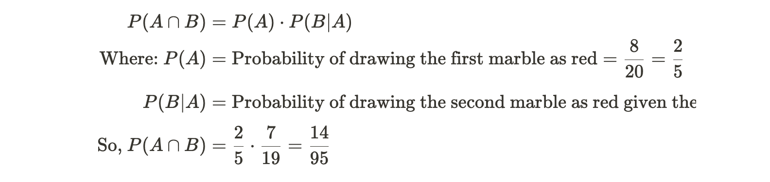
a. You have a bag of 20 marbles, 8 of which are red, and 12 are blue. You draw one marble from the bag, record its color (Event A), and then draw a second marble from the same bag without replacement and record its color (Event B). Calculate the probability that both marbles are red (Event A and Event B).

Solution:

b. Consider a situation where you are predicting the outcome of a soccer match (win, lose, or draw) for your favorite team (Event A) based on their performance history. Given that your team lost the last three matches (Event B), calculate the conditional probability that they will win the next match (P(A|B)).

Solution:

To calculate the conditional probability that your favorite team will win the next match (Event A) given that they lost the last three matches (Event B), you can use the following formula:

Since the outcomes of soccer matches can be influenced by various factors, let's assume values for P(A_∩_B) and P(B) based on your knowledge or data. For example, if you estimate that your team wins 20% of the time (A), and they lost the last three matches (B), you can calculate:

To get the specific value of P(A_∣_B), you would need to provide the probability P(B) based on your assessment of your team's performance and the factors affecting the matches.

Bayes' Theorem Introduction:

Bayes' Theorem is a fundamental concept in probability theory and statistics that provides a way to update the probability for a hypothesis as more evidence or information becomes available. It is named after the 18th-century British statistician and theologian Thomas Bayes, although the theorem itself was published posthumously in 1763 by his friend Richard Price.

Historical Context and Significance:

The historical context of Bayes' Theorem is quite interesting. Thomas Bayes developed the theorem to address a problem related to inverse probability, which was a topic of great interest in the 18th century. Inverse probability problems involve determining the probability of a cause based on the observed effects, which is essentially what Bayes' Theorem accomplishes.

Bayes' Theorem remained relatively obscure until Richard Price rediscovered and published it. It gained significant attention because it provided a formal mathematical framework for updating beliefs or probabilities when new evidence is obtained. This was particularly important in fields like astronomy, where it could be used to refine predictions about celestial bodies' positions based on new observations.

Relevance in Various Fields:

Bayes' Theorem is of immense importance and applicability in various fields:

1. Statistics: In statistics, Bayes' Theorem is a cornerstone of Bayesian statistics. It allows statisticians to update their beliefs about parameters or hypotheses based on observed data. Bayesian statistics is especially useful when dealing with small or incomplete datasets, and it's employed in fields like finance, epidemiology, and social sciences.
2. Machine Learning: Bayes' Theorem plays a crucial role in machine learning algorithms, particularly in Bayesian machine learning. It's used for tasks like spam email filtering, document classification, and reinforcement learning. Bayesian methods provide a probabilistic framework for modeling uncertainty and making predictions.
3. Medical Diagnosis: In medical diagnosis, Bayes' Theorem can help determine the probability of a patient having a particular disease based on symptoms and test results. It's a fundamental tool in medical decision support systems, where accurate diagnosis and treatment planning are critical.
4. Natural Language Processing: In NLP, Bayes' Theorem is used in algorithms like Naive Bayes for text classification and sentiment analysis. It helps classify documents or texts into categories based on word frequencies and probabilities.
5. Finance: In finance, Bayes' Theorem is used for risk assessment, portfolio management, and fraud detection. It enables financial analysts to update their predictions and make informed decisions based on changing market conditions.
6. Astronomy: As mentioned earlier, Bayes' Theorem has historical significance in astronomy for predicting celestial events and improving our understanding of the universe.

Bayes' Theorem Formula:

Bayes' Theorem, in its general form, is a mathematical formula used in probability theory and statistics to update the probability of a hypothesis or event based on new evidence. It is expressed as:

P(A_∣_B)=P(B_∣_A)⋅_P_(A)/ P(B)

Where:

• P(A_∣_B) is the posterior probability of event or hypothesis A given the evidence B.
• P(B_∣_A) is the likelihood, representing the probability of observing evidence B if hypothesis A is true.
• P(A) is the prior probability, representing the initial probability of hypothesis A before considering the evidence.
• P(B) is the probability of the evidence B occurring, also known as the marginal likelihood.

Components of the Formula:

1. Prior Probability (P(A)): This is the initial probability assigned to the hypothesis A before taking into account any new evidence. It represents our belief or knowledge about A before observing the evidence B. The prior probability reflects any relevant background information or historical data.
2. Likelihood (P(B∣A)): The likelihood measures the probability of observing the evidence B given that the hypothesis A is true. It quantifies how well the hypothesis A explains or predicts the evidence B. The likelihood is often derived from data or domain-specific models.
3. Evidence (P(B)): The evidence is the probability of observing the evidence B without any regard to a specific hypothesis. It serves as a normalizing factor and ensures that the posterior probability is a valid probability distribution. It is calculated as the sum of the product of the likelihood and prior probability for all possible hypotheses:

Where Ai represents all possible hypotheses.

4. Posterior Probability (P(A∣B)): This is the updated probability of hypothesis A after taking into account the new evidence B. It represents our revised belief about A in light of the evidence. The posterior probability is the quantity of interest in Bayesian reasoning, as it provides a way to update and refine our beliefs based on new information.

Role of Each Component in Bayesian Reasoning:

• The prior probability reflects our initial beliefs or knowledge and sets the starting point for the analysis. It incorporates existing information into the analysis.
• The likelihood assesses how well the hypothesis explains the observed evidence. It quantifies the strength of the relationship between the hypothesis and the evidence.
• The evidence ensures that the posterior probability is a valid probability distribution by normalizing the result. It accounts for all possible ways the evidence could occur.
• The posterior probability is the ultimate goal of Bayesian reasoning. It represents our updated belief or understanding of the hypothesis after considering the evidence. It combines prior knowledge with new information to provide a more accurate estimate of the hypothesis's probability.

Bayes' Theorem is a fundamental tool for making decisions, predictions, and inferences in various fields, allowing for the incorporation of new data and evidence into existing knowledge or beliefs. It forms the basis of Bayesian statistics and reasoning.

Applications of Bayes' Theorem:

Bayes' Theorem is applied in various real-world scenarios to make informed decisions, particularly when new evidence is available. Here are practical examples in different fields:

1. Medical Diagnosis:
   • Breast Cancer Diagnosis: Bayes' Theorem is used in breast cancer screening. Given a woman's age and mammogram results, it can calculate the probability of having breast cancer. New evidence, such as additional diagnostic tests, can be incorporated to update the probability and make more accurate diagnoses.
2. Spam Email Filtering:
   • Email Classification: In spam email filtering, Bayes' Theorem helps classify emails as spam or not spam based on the presence of certain keywords or patterns. The likelihood of a word appearing in spam and non-spam emails is used to update the prior probability that an email is spam, resulting in improved filtering accuracy.
3. Forensic Science:
   • DNA Evidence: In forensic science, Bayes' Theorem is used to calculate the probability of a suspect's DNA matching DNA found at a crime scene. It combines prior information about the suspect's DNA profile with the likelihood of the observed DNA evidence matching that profile.
4. Machine Learning:
   • Natural Language Processing: In sentiment analysis, Bayes' Theorem is applied to classify text as positive or negative sentiment based on the frequency of certain words. It updates the probability that a given document expresses a particular sentiment as new evidence (words) is observed.
5. Epidemiology:
   • Disease Outbreak Prediction: Bayes' Theorem can be used to predict disease outbreaks. The prior probability of an outbreak is updated with new data, such as the number of reported cases and population movement, to estimate the current risk of an epidemic.
6. Finance:
   • Portfolio Management: Bayes' Theorem is applied to manage investment portfolios. It can help investors update their beliefs about asset returns based on new economic data, company reports, or market trends, aiding in portfolio adjustments.
7. Quality Control:
   • Manufacturing Defects: In manufacturing, Bayes' Theorem is used to estimate the probability of a product having a defect given certain test results. This helps in making decisions about whether to accept or reject a batch of products.

Role in Updating Probabilities:

In all these applications, Bayes' Theorem plays a central role in updating probabilities based on new evidence. It allows for a systematic way to combine prior knowledge or beliefs with observed data to obtain more accurate and up-to-date probabilities. This updating process is particularly valuable when dealing with uncertainty and making decisions in dynamic and evolving situations. By incorporating new evidence, Bayes' Theorem helps individuals and organizations make more informed choices and predictions.

Bayesian Inference:

Bayesian inference is a broader statistical concept built upon Bayes' Theorem. While Bayes' Theorem provides a mathematical framework for updating probabilities based on new evidence, Bayesian inference is the entire process of using this framework to make probabilistic inferences, model data, estimate parameters, and make predictions. It encompasses a systematic approach to statistical reasoning that incorporates prior knowledge and evidence to draw conclusions.

Using Bayesian Inference for Statistical Modeling and Parameter Estimation:

Bayesian inference is particularly powerful for statistical modeling and parameter estimation because it allows practitioners to:

1. Incorporate Prior Knowledge: Bayesian inference allows the incorporation of prior information or beliefs into statistical analyses. This is especially valuable when dealing with small datasets or situations where prior knowledge can provide important context.
2. Update Beliefs: As new data becomes available, Bayesian inference updates the initial beliefs (represented by prior probabilities) using Bayes' Theorem. This updating process leads to posterior probability distributions that reflect updated beliefs based on observed evidence.
3. Quantify Uncertainty: Bayesian inference provides a natural way to quantify uncertainty in statistical estimates. Instead of producing point estimates, it yields entire probability distributions for parameters or model predictions. This allows for a more nuanced understanding of uncertainty.
4. Model Complexity: Bayesian models can be as simple or complex as needed. They can include multiple parameters, hierarchical structures, and various forms of data likelihoods, making them suitable for a wide range of modeling tasks.
5. Model Selection: Bayesian inference supports model selection by comparing different models' posterior probabilities. This helps in choosing the most appropriate model for a given dataset.

Examples of Bayesian Inference in Action:

1. Medical Trials: Bayesian inference is used in clinical trials to estimate the effectiveness of a new drug. Prior information about similar drugs or treatments can be incorporated, and as more patients are enrolled and data collected, the posterior distribution of the drug's efficacy is continuously updated.
2. Weather Forecasting: Bayesian inference is applied in weather forecasting to update predictions as new weather data is collected. Prior knowledge about seasonal patterns and climate conditions can be integrated into the models, and the forecasts are continually adjusted based on real-time observations.
3. Machine Learning: Bayesian inference is used in machine learning, particularly in Bayesian networks and probabilistic graphical models. It helps in probabilistic reasoning, classification, and making predictions while taking into account uncertainty in the data.
4. Natural Language Processing: In language modeling, Bayesian inference can be applied to estimate the probability of a word or phrase occurring in a sentence. This is useful in tasks such as speech recognition and text generation.
5. Finance: Bayesian inference is used in finance for risk management and portfolio optimization. It helps investors update their beliefs about asset returns and make informed decisions in dynamic financial markets.

In essence, Bayesian inference provides a powerful and flexible framework for modeling complex systems, estimating parameters, and making predictions while accounting for uncertainty. It is widely employed in fields where probabilistic reasoning and the incorporation of prior knowledge are essential for making informed decisions.

Conditional Probability vs. Bayes' Theorem:

Conditional probability and Bayes' Theorem are related concepts in probability theory, but they serve different purposes and address different aspects of probabilistic reasoning.

Conditional Probability:

Definition: Conditional probability is the probability of one event occurring given that another event has already occurred. It answers the question: "What is the likelihood of event A happening, given that we know event B has occurred?"

Notation: It is denoted as P(A_∣_B), read as "the probability of A given B."

Formula: The formula for conditional probability is:

P(A_∣_B)=P(A_∩_B)/P(B)

Here, P(A_∩_B) is the joint probability of both events A and B happening together, and P(B) is the probability of event B.

Use: Conditional probability is used to understand how one event's occurrence or knowledge about it affects the probability of another event. It's fundamental in scenarios like medical diagnosis, risk assessment, and many real-life decision-making processes.

Bayes' Theorem:

Definition: Bayes' Theorem is a specific mathematical tool used for updating probabilities when new evidence becomes available. It answers the question: "What is the probability of a hypothesis or event A being true, given new evidence B?"

Notation: In the context of Bayes' Theorem, P(A) represents the prior probability of event A before considering evidence B, P(B_∣_A) is the likelihood of observing evidence B if A is true, P(B) is the probability of observing evidence B, and P(A_∣_B) is the posterior probability of A given B.

Formula: The formula for Bayes' Theorem is:

(A_∣_B)=P(B_∣_A)⋅_P_(A)/ P(B)

Use: Bayes' Theorem is employed when you want to update your beliefs or probabilities about a hypothesis or event in light of new evidence. It is commonly used in fields like statistics, machine learning, medical diagnosis, and decision analysis.

Key Distinction:

The key distinction is that conditional probability deals with the likelihood of events occurring given other events, without necessarily involving prior beliefs or updating. It helps answer questions like "What is the probability of rain given that it's cloudy?"

In contrast, Bayes' Theorem specifically addresses the updating of probabilities or beliefs based on new evidence. It is a tool for incorporating prior knowledge (prior probability) and new information (likelihood and evidence) to arrive at an updated probability (posterior probability) for an event or hypothesis. It helps answer questions like "What is the probability of a medical condition given a positive test result?"

While both concepts deal with probabilities and conditional relationships, Bayes' Theorem is a more versatile tool for Bayesian reasoning and updating probabilities in dynamic situations.

Limitations and Challenges:

a. Accurate Prior Probabilities:

• Challenge: Bayes' Theorem heavily relies on prior probabilities, which represent existing beliefs or knowledge. Obtaining accurate prior probabilities can be challenging, especially when dealing with complex or poorly understood phenomena.
• Solution: Sensitivity analysis, where different prior probabilities are considered, can help assess how much results depend on prior assumptions.

b. Data Availability and Quality:

• Challenge: Bayesian inference relies on observed data to update probabilities. Inadequate or biased data can lead to incorrect conclusions. In some cases, data may be limited or expensive to collect.
• Solution: Careful data collection, cleaning, and validation are essential. Bayesian methods can also handle small datasets through informative priors.

c. Computational Complexity:

• Challenge: For complex models, Bayesian inference can be computationally intensive. Calculating posterior distributions analytically may not be feasible.
• Solution: Techniques like Markov Chain Monte Carlo (MCMC) can be employed to approximate posterior distributions for complex models.

d. Model Misspecification:

• Challenge: If the model used in Bayesian analysis does not accurately represent the underlying reality, the results may be misleading.
• Solution: Model checking and validation are critical. Sensitivity analysis can help assess the impact of model assumptions on results.

e. Misconceptions and Misuses:

• Challenge: Bayes' Theorem is sometimes misused or misunderstood. For example, assuming that a low prior probability implies a low posterior probability, which is not always the case.
• Solution: Promote proper understanding and use of Bayes' Theorem through education and awareness of its limitations.

Advanced Topics:

a. Bayesian Networks:

• Description: Bayesian networks are graphical models that represent probabilistic relationships among a set of variables. They are used for reasoning under uncertainty, decision analysis, and causal inference.
• Application: Bayesian networks are applied in fields like healthcare (diagnosis and treatment planning), finance (risk assessment), and artificial intelligence (knowledge representation and reasoning).

b. Markov Chain Monte Carlo (MCMC) Methods:

• Description: MCMC methods are used for sampling from complex probability distributions, especially when analytical solutions are unavailable. They are widely used in Bayesian statistics to approximate posterior distributions.
• Application: MCMC methods are applied in Bayesian modeling, Bayesian parameter estimation, and Bayesian model selection.

c. Hierarchical Bayesian Modeling:

• Description: Hierarchical Bayesian modeling extends Bayesian analysis by modeling variability at multiple levels. It's particularly useful when data hierarchies exist.
• Application: Hierarchical Bayesian models are used in ecology (modeling species abundance at different sites), psychology (modeling individual and group-level behavior), and economics (modeling individual and regional economic trends).

These advanced topics expand upon the foundational concepts of conditional probability and Bayes' Theorem, allowing for more sophisticated and powerful applications in various domains. However, they also come with their own complexities and challenges, such as model complexity and computational demands. Understanding these advanced topics can lead to more nuanced and accurate probabilistic modeling and inference.

Conclusion

Conditional probability and Bayes' Theorem are foundational concepts in probability theory and statistics. Conditional probability allows us to assess the likelihood of events given other events, while Bayes' Theorem provides a systematic way to update probabilities based on new evidence. These concepts find widespread applications in fields ranging from healthcare to finance, enabling more accurate predictions, informed decisions, and probabilistic reasoning.

Key Takeaways

1. Conditional probability assesses the likelihood of one event occurring given another event has already happened, vital for making context-aware predictions.
2. Bayes' Theorem extends conditional probability by incorporating prior beliefs, updating them with new evidence, and quantifying uncertainty.
3. Applications of Bayes' Theorem include medical diagnosis, spam email filtering, forensic science, and machine learning, enabling informed decision-making in dynamic environments.
4. Bayesian inference, built on Bayes' Theorem, supports parameter estimation, model selection, and complex probabilistic modeling by integrating prior knowledge and observed data.
5. Challenges in applying Bayes' Theorem include obtaining accurate prior probabilities, data quality, computational complexity, model validity, and addressing misconceptions or misuses.

Practice Questions

1. Assume P(A)=0.2, P(B)=0.6,P(A U B)=0.5, Then P[A|B]=

a. 0.2

b. 0.3

c. 0.6

d. 0.5

Answer:

(D)

Explaination:

Conditional Probability formula :-   P (A |  B)  = P( A ∩ B ) / P ( B )

Inclusion exclusion principle  :-   P ( A U B ) =   P( A ) + P( B ) – P( A ∩ B )

0.5 =  0.2  +  0.6 –  P( A ∩ B )

P( A ∩ B ) = 0.3

Given Data :-    P( A )  = 0.2   ,    P( B )  =  0.6

Put all the value in conditional probability formula

P (A |  B)  =   0.3 / 0.6  = 0.5

So option D is true

2. Suppose that a shop has an equal number of LED bulbs of two different types. The probability of an LED bulb lasting more than 100 hours given that it is of Type 1 is 0.7, and given that it is of Type 2 is 0.4. The probability that an LED bulb chosen uniformly at random lasts more than 100 hours is :

a. 0.55

b. 0.7

c. 0.4

d. 0.35

Answer:

(A)

Explanation:

The question is based on Bayes’ Theorem.

P(LED is Type 1) = 1/2

P(LED is type 2) = 1/2

Now, we need to see conditional probabilities.

P( LED lasting more than 100 hours / LED is Type 1) = 0.7

P( LED lasting more than 100 hours / LED is Type 2) = 0.4

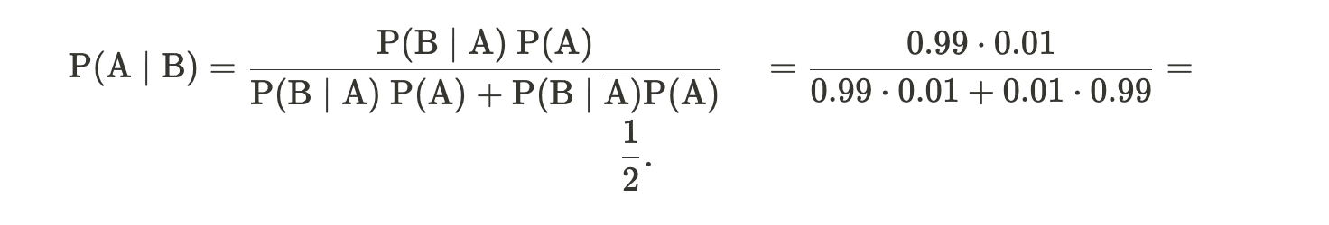
3. Suppose a test is 99% accurate and 1% of people have a disease. What is the probability that you have the disease given that you tested positive?   a. 1/2 b. 2/3 c. 1/4 d. 3/4

Solution:

Let B be the event of testing positive and A be the event of having the disease.

We want to figure out P(A∣B). We know P(B∣A)=0.99 , which tells us we should use Bayes Theorem. Then, we also know  P(B∣A’) = 0.01  and P(A)=0.01,P(A’)=0.99. We can plug this into the formula to get

4.

Given that they passed the exam what is the probability it is a woman ?

Answer:

• What is the probability of having a woman ; 100/200 and it's equal to 0.5
• What is the probability of passing the exam ; 169/200 and it's equal to 0.845
• The probability of a woman passing the exam is 92/100 and it's equal to 0.92
• P(A|B) = (P(0.5) x P(0.92 ) / P(0.845)
• P(A|B) = 0.54
• 92/169 = 0.54 too

5. Covid 19 has taken over the world and the use of Covid19 tests is still relevant to block the spread of the virus and protect our families.

You can follow the statistics of Covid 19 on the World Health Organization website: https://covid19.who.int/

If the Covid19 infection rate is 10% of the population, and thanks to the tests we have in Algeria, 95% of infected people are positive with 5% false positive.

What would be the probability that I am really infected if I test positive?

Solution :

Parameters :

• 10% infected
• 95% Test positive while infected
• 5% False positive while non infected
• 90% not infected

We will start multiplying the probability of infection (10%) by the probability of testing positive given that be infected (95%) then we divided by the sum of the probability of infection (10%) by the probability of testing positive given that be infected ( 95%) with not infected (90%) multiplied by false positive (5%)

• P(A|B) = P(A) * P(B|A) / Σ P(A) * P(B|A)
• P(A|B) = 0.1 * 0.95 /(0.95 * 0.1) +(0.05*0.90)
• P(A|B) = 0.095 / 0.095 + 0.045
• P(A|B) = 0.678