Introduction to Vectors and Matrices for GATE Exam

Vectors and matrices are fundamental mathematical concepts with widespread importance in various fields of science and engineering.

They provide a structured way to represent and manipulate data, making them essential tools in the following areas:

1. Physics: Vectors are crucial for describing physical quantities like force, velocity, and acceleration. They simplify the analysis of complex systems and are central to classical mechanics and electromagnetism.
2. Engineering: Vectors and matrices are used extensively in engineering for tasks such as structural analysis, circuit design, and signal processing. They enable engineers to model and solve real-world problems efficiently.
3. Computer Graphics: Vectors are fundamental for describing the position and orientation of objects in 2D and 3D space, making them essential for computer graphics, video game development, and animation.
4. Machine Learning and Data Science: Matrices are fundamental for representing datasets, and linear algebra operations on matrices underlie many machine learning algorithms, including neural networks and dimensionality reduction techniques.
5. Economics and Finance: Matrices are used in economic models to represent input-output relationships and solve systems of equations. In finance, they play a crucial role in portfolio optimization and risk assessment.
6. Chemistry and Biology: Vectors and matrices are used in molecular modeling, quantum mechanics, and bioinformatics for analyzing and simulating complex molecular structures and biological data.
7. Statistics: Matrices are used in multivariate statistics for data analysis, hypothesis testing, and regression analysis, enabling researchers to work with high-dimensional datasets.
8. Civil and Mechanical Engineering: Vectors and matrices are employed in finite element analysis to simulate and optimize the behavior of structures and mechanical systems.
9. Electrical Engineering: Matrices are essential for circuit analysis and control systems, allowing engineers to design and analyze electrical circuits and control systems.
10. Operations Research: Linear programming, a common optimization technique in operations research, relies heavily on matrices and vectors to model and solve complex resource allocation problems.

Here's a breakdown of their significance:

Vectors

1. Representation of Quantities: Vectors are used to represent quantities that have both magnitude and direction. In physics, for example, velocity and force are represented as vectors because they not only have a value but also a specific direction in space.
2. Geometric Interpretation: Vectors can be thought of as directed line segments, connecting points in space. This geometric interpretation is crucial in fields like geometry, computer graphics, and engineering.
3. Mathematical Operations: Vectors can be added, subtracted, scaled (multiplied by a scalar), and subjected to various mathematical operations like dot and cross products. These operations are fundamental in physics, engineering, and linear algebra.

Matrices

1. Structured Data Representation: Matrices are rectangular arrays of numbers, symbols, or data. They are used to represent structured data, such as spreadsheets, images, and databases, where data is organized into rows and columns.
2. Linear Transformations: Matrices are central to linear algebra, where they represent linear transformations. These transformations are essential in various fields, from computer graphics (transforming 3D objects) to physics (representing quantum states).
3. Systems of Equations: Matrices are employed to solve systems of linear equations efficiently. This is crucial in solving real-world problems in engineering, physics, and economics, where multiple variables are interrelated.
4. Data Manipulation: In data science, machine learning, and statistics, matrices are used to represent datasets, making it possible to perform operations like matrix multiplication and inversion to analyze and model complex data.

Both vectors and matrices offer a structured way to organize and manipulate data, making them indispensable in numerous applications. They provide a common mathematical language that bridges the gap between theory and practical problem-solving, allowing researchers and engineers to work with complex data and systems effectively.

What are Vectors?

A. Definition of a Vector:

A vector is a mathematical object that represents a quantity with both magnitude and direction. It is often depicted as an arrow in space, where the length of the arrow represents the magnitude of the quantity, and the direction of the arrow indicates the direction of the quantity. Vectors can be used to represent various physical quantities, such as:

1. Displacement: In physics, a vector can represent the change in position of an object, specifying both how far and in which direction it has moved.
2. Velocity: Vectors can represent the speed and direction of an object's motion.
3. Force: Force vectors describe the strength and direction of forces acting on an object.
4. Acceleration: Vectors can represent the rate of change of velocity, including its direction.
5. Momentum: In physics, momentum is a vector quantity that combines an object's mass and velocity.
6. Electric and Magnetic Fields: Vectors are used to represent the strength and direction of electric and magnetic fields in electromagnetism.
7. Wind Velocity: In meteorology, vectors are employed to describe the speed and direction of wind.

In mathematical notation, a vector is often denoted using a bold lowercase letter (e.g., v) or an arrow above the letter (e.g., v->). Vectors can also be represented as ordered lists of numerical components, such as (x, y, z) in three-dimensional space, where each component represents the magnitude of the vector along a specific axis.

Vectors can be added, subtracted, scaled (multiplied by a scalar), and subjected to various mathematical operations, making them a fundamental concept in linear algebra and a valuable tool for solving problems in physics, engineering, computer graphics, and many other fields.

B. Vector Notation:

Vector notation is a way of representing vectors using variables and mathematical symbols. In this notation, a vector is typically denoted by a letter with an arrow on top or a boldface letter to distinguish it from scalar quantities (which have only magnitude). Let's introduce vector notation using the variable "v" as an example:

1. Notation with an Arrow (v->):

• A vector is often represented with an arrow on top of the variable, like “v->” to indicate its direction.
• For example, if "v->" represents a velocity vector, it means that the object is moving in a specific direction with a certain speed.

2. Boldface Notation (????):

• In some texts and contexts, vectors are represented using boldface letters, such as ????, to distinguish them from scalars (e.g., v for speed).
• This notation is common in mathematical literature and computer programming, where adding arrows may not be feasible.

Now, let's discuss how vectors are typically represented with arrows in diagrams:

• Geometric Representation with Arrows:
  • In diagrams and illustrations, vectors are often depicted as arrows in space.
  • The length of the arrow represents the magnitude (or size) of the vector, and the direction of the arrow indicates the vector's direction.
  • For example, if you have a velocity vector "v->" with a length of 5 units pointing east, you would draw an arrow 5 units long in the eastward direction.
  • The arrow's starting point is usually not significant; what matters is the arrow's length and direction.
• Coordinate Axes:
  • In three-dimensional space, vectors can be related to the coordinate axes (x, y, z).
  • A vector "v->" can be represented as (x, y, z), where x, y, and z are the components of the vector along each axis.
  • For example, if you have a position vector (3, 4, 1), it means the vector extends 3 units along the x-axis, 4 units along the y-axis, and 1 unit along the z-axis.

Vectors are a fundamental concept in mathematics and science, and their notation and representation with arrows simplify the visualization and understanding of quantities that have both magnitude and direction. They play a crucial role in physics, engineering, and many other fields where describing and manipulating directional quantities is essential.

C. Components of a Vector:

Breaking down a vector into its components along different axes, such as x, y, and z in three-dimensional space, is a fundamental concept in vector analysis. This process allows us to understand how much of the vector's magnitude lies in each direction. Here's how it's done:

1. Components Along the Axes:

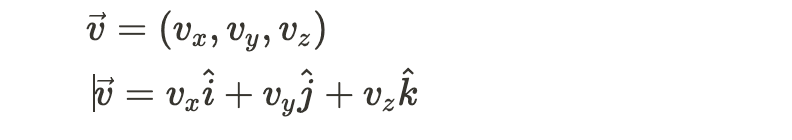
• Let's say you have a vector $\vec{v}$ in three-dimensional space. This vector can be thought of as a combination of three components along the x, y, and z axes.

2. Vector Notation:

• vx is the component of v→ along the x-axis.
• vy is the component of v→ along the y-axis.
• vz is the component of v→ along the z-axis.

3. Magnitude and Direction:

• The magnitudes of these components, vx, vy, and vz, represent how much of the vector's magnitude lies in each respective direction.
• The direction of each component is aligned with its respective axis.

4. Vector Addition:

• To reconstruct the original vector v->, you can add its components together using vector addition. The vector addition rule is as follows:

where:

• i^ is the unit vector along the x-axis (1, 0, 0).
• j^ is the unit vector along the y-axis (0, 1, 0).
• k^ is the unit vector along the z-axis (0, 0, 1).
• So, you can think of the vector v-> as the sum of its components along each axis, each multiplied by the respective unit vector.

5. Magnitude of the Components:

You can find the magnitudes of the components vx, vy, and vz, using the Pythagorean theorem. For example, the magnitude of vx is given by:

This process of breaking a vector into its components along different axes is particularly useful in physics, engineering, and other fields. It allows you to analyze complex motions, forces, or physical quantities in a simplified manner by considering their contributions along specific directions. It's also essential for solving problems involving coordinate systems and vector mathematics.

Vector Operations

A. Addition and Subtraction:

Vectors can be added and subtracted using well-defined rules, which are fundamental operations in vector mathematics. These operations allow you to combine vectors to find their resultant vector (sum) or the vector between two points (difference). Here's how vector addition and subtraction work:

Vector Addition:

When adding two vectors, you essentially combine their effects, taking into account both their magnitudes and directions. To add vectors A-> and B->:

Graphical Method:

• Draw both vectors on a coordinate system so that their tails (starting points) coincide.
• The resultant vector R-> is then drawn from the tail of A-> to the tip of B-> (or vice versa).
• R-> represents the sum of A-> and B-> in terms of magnitude and direction.

Component Method:

• Break down each vector into its components along the coordinate axes. For example,

• Add the corresponding components together to get the components of the resultant vector:

Vector Subtraction:

Vector subtraction is essentially vector addition with a negation. To subtract vector B-> from vector A->:

1. Negative Vector:
   • Find the negative of B-> by reversing its direction. This is done by changing the direction of B-> but keeping its magnitude the same, resulting in B->.
2. Addition Method:
   • Add vector A-> and B-> using the vector addition method described earlier.
   • The resultant vector R-> represents the difference between A-> and B->.

Examples:

Let's consider a couple of examples:

Vector Addition:

• Suppose you have a vector A-> = (3, 2) and another vector B-> = (1, -1).
• Using the component method, you can add these vectors as follows: R-> = (3 + 1, 2 - 1) = (4, 1).
• So, the resultant vector R-> is (4, 1).

Vector Subtraction:

• Consider vector A-> = (5, 3) and vector B-> = (2, 1).
• To find the difference, you first find the negative of B-> : B-> = (-2, -1).
• Now, you add A-> and B->: R-> = (5, 3) + (-2, -1) = (5 - 2, 3 - 1) = (3, 2).
• So, the resultant vector R-> is (3, 2).

These examples demonstrate how to perform vector addition and subtraction by combining their components along the respective axes. The graphical method and component method are both valid ways to perform these operations, depending on the given vectors and the problem's context.

B. Scalar Multiplication:

Scalar multiplication is a fundamental operation involving vectors and scalars (which are simply numerical values without direction). When you multiply a vector by a scalar, you change the magnitude of the vector while preserving its direction (if the scalar is positive) or reversing its direction (if the scalar is negative). Here's a more detailed explanation:

Scalar Multiplication Effect on a Vector:

1. Scalar Greater than 1: If you multiply a vector by a scalar greater than 1, you increase the vector's magnitude while keeping its direction unchanged. This results in a vector that points in the same direction as the original but is longer.
2. Scalar Between 0 and 1: When multiplying a vector by a scalar between 0 and 1, you decrease the vector's magnitude while maintaining its direction. This results in a vector that points in the same direction as the original but is shorter.
3. Scalar Equal to 0: Multiplying a vector by 0 results in a vector with zero magnitude. In other words, it's a vector at the origin, having no length or direction.
4. Negative Scalar: If you multiply a vector by a negative scalar, you reverse the vector's direction while keeping the magnitude unchanged. This results in a vector pointing in the opposite direction of the original.

Examples of Scalar Multiplication:

Let's illustrate scalar multiplication with some examples:

1. Increasing Magnitude:
   • Suppose you have a vector v-> = (2, 3), and you multiply it by the scalar 4: v->.
   • The result is v-> = (4 * 2, 4 * 3) = (8, 12).
   • The original vector's direction remains the same, but its magnitude increases fourfold.
2. Decreasing Magnitude:
   • Take the same vector v-> = (2, 3) and multiply it by the scalar 0.5: $0.5\vec{v}$.
   • The result is 0.5v-> = (0.5 * 2, 0.5 * 3) = (1, 1.5).
   • The original vector's direction remains unchanged, but its magnitude is halved.
3. Reversing Direction:
   • Consider vector w-> = (4, -2), and multiply it by the scalar -1:
   • The result is w-> = (-1 * 4, -1 * -2) = (-4, 2).
   • The direction of the original vector is reversed, while its magnitude remains the same.
4. Zero Scalar:
   • If you multiply any vector by 0, the result is always the zero vector: 0v-> = (0, 0).
   • This vector has no magnitude or direction and is located at the origin.

Scalar multiplication is a powerful concept used in various applications, such as scaling objects in computer graphics, changing the intensity of forces in physics, and rescaling data in data analysis and machine learning. It allows you to adjust the magnitude of a vector while preserving or reversing its direction as needed.

C. Dot Product:

Dot Product (Scalar Product) of Two Vectors:

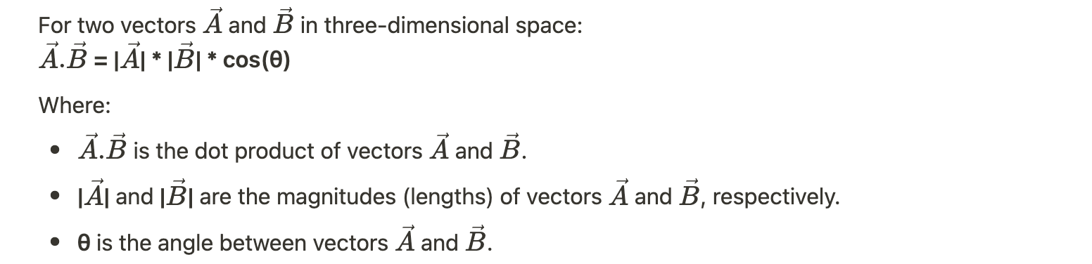
The dot product, also known as the scalar product, is a mathematical operation that takes two vectors and produces a scalar (a single numerical value). It is denoted by a dot (·) between the vectors and is defined as follows:

Geometric Interpretation:

The dot product has a geometric interpretation that provides insight into its significance:

1. Scalar Projection: The dot product represents the length of the projection of vector A-> onto vector B-> (or vice versa) when the vectors are placed tail-to-tail.
2. Angle Measurement: It measures how much of vector A-> points in the direction of vector B->, scaled by the magnitude of both vectors and the cosine of the angle between them.

Computing the Dot Product:

To compute the dot product between two vectors $\vec{A}$ and $\vec{B}$, follow these steps:

1. Find the magnitudes of both vectors: |$\vec{A}$| and |$\vec{B}$|.
2. Determine the angle θ between the vectors. You can use trigonometric functions or vector properties to find the angle.
3. Use the formula:

Properties of the Dot Product:

The dot product of vectors has several important properties:

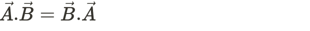
1. Commutative:

• The order of multiplication does not affect the result.

2. Distributive over Addition:

• The dot product distributes over vector addition.

3. Scalar Multiplication:

• You can factor out scalars from one of the vectors in the dot product.

4. Orthogonal Vectors: If the dot product of two vectors is zero, it implies that the vectors are orthogonal (perpendicular) to each other.

5. Angle between Vectors:

• If the dot product is positive, the angle between the vectors is acute (less than 90 degrees).
• If the dot product is negative, the angle between the vectors is obtuse (greater than 90 degrees).
• If the dot product is zero, the vectors are orthogonal.

The dot product is a versatile tool used in various fields, including physics, engineering, and geometry, to analyze relationships between vectors, determine angles, calculate work, and find projections.

Examples of Dot Product:

Example 1: Finding Work Done Suppose you have a force vector F-> = (3, 4) Newtons applied to an object and a displacement vector d-> = (2, 1) meters. To find the work done by the force as the object is moved along the displacement:

Calculate the magnitudes:

• |F->| = √(3² + 4²) = 5 Newtons
• |d->| = √(2² + 1²) = √5 meters

Calculate the angle θ between the vectors:

• cos(θ) = (F->.d->) / (|F->| * |d->|)
• cos(θ) = (3 * 2 + 4 * 1) / (5 * √5) = (6 + 4) / (5 * √5) = 10 / (5 * √5) = 2 / √5

Calculate the work:

• Work = 5 * √5 * 2 / √5 = 10 Joules

So, the work done by the force in moving the object is 10 Joules.

Example 2: Checking Orthogonality Suppose you have two vectors A-> = (1, 2) and B-> = (-2, 1). To determine whether these vectors are orthogonal (perpendicular), calculate their dot product:

A->.B-> = 1 * (-2) + 2 * 1 = -2 + 2 = 0

Since the dot product is zero, the vectors A-> and B-> are orthogonal to each other.

Example 3: Finding the Angle Between Vectors Given two vectors X-> = (3, 4) and Y-> = (1, -1), you can find the angle between them using the dot product:

1. Calculate the magnitudes:
   • |X->| = √(3² + 4²) = 5 units
   • |Y->| = √(1² + (-1)²) = √2 units
2. Calculate the dot product:
   • X->.Y-> = 3 * 1 + 4 * (-1) = 3 - 4 = -1
3. Calculate the cosine of the angle:
   • cos(θ) = (-1) / (5 * √2)
4. Find the angle:
   • θ = arccos(-1 / (5 * √2))

Using a calculator, you can determine that θ ≈ 108.43 degrees.

These examples demonstrate the versatility of the dot product in various contexts, including calculating work, checking orthogonality, and finding angles between vectors.

D. Cross Product:

Cross Product (Vector Product) of Two Vectors:

The cross product is a mathematical operation that takes two vectors and produces a third vector that is orthogonal (perpendicular) to the plane formed by the original vectors. It is denoted by a cross (×) between the vectors and is defined as follows:

Where:

• A-> x B-> is the cross product of vectors A-> and B->.
• |A->| and |B->| are the magnitudes (lengths) of vectors A-> and B->, respectively.
• θ is the angle between vectors A-> and B->.
• n^ is the unit vector perpendicular to the plane formed by A-> and B->. The direction of n^ follows the right-hand rule.

Geometric Interpretation:

The cross product has a geometric interpretation that provides insight into its significance:

1. Direction: The resulting vector points in a direction that is perpendicular to the plane containing the original vectors A-> and B->.
2. Magnitude: The magnitude of the resulting vector is equal to the area of the parallelogram formed by A-> and B-> when their tails are placed at the same point.
3. Right-Hand Rule: To determine the direction of the resulting vector, use the right-hand rule: If you curl your fingers from vector A-> to vector B->, your thumb points in the direction of the cross product vector A-> and B->.

Computing the Cross Product:

To compute the cross product between two vectors A-> and B->, follow these steps:

1. Calculate the magnitudes of both vectors: |A->| and |B->|.
2. Determine the angle θ between the vectors. You can use trigonometric functions or vector properties to find the angle.
3. Calculate the cross product using the formula:

Properties of the Cross Product:

The cross product of vectors has several important properties:

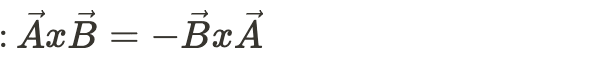
1. Anticommutative:

• The order of multiplication affects the result, and the cross product is anticommutative.

2. Distributive over Addition:

• The cross product distributes over vector addition.

3. Magnitude of the Cross Product:

• The magnitude of the cross product is given by:

• It represents the area of the parallelogram formed by the vectors.

4. Direction of the Cross Product: The direction is perpendicular to the plane formed by A-> and B-> and follows the right-hand rule.

The cross product is a valuable mathematical tool used in physics, engineering, and other fields for tasks such as calculating torque, finding the normal vector of a plane, and determining angular momentum. It provides information about both direction and magnitude in a way that is distinct from the dot product.

Examples of Cross Product:

Example 1: Calculating Torque

Suppose you have a lever arm represented by vector r-> and a force vector F-> applied to the lever arm. To calculate the torque (rotational force) produced by the force about a pivot point, you can use the cross product:

1. Vectors: Consider the following vectors:
   • r-> = (3, 2, 0) meters (represents the position of the force application relative to the pivot).
   • F-> = (5, -1, 0) Newtons (represents the force applied).
2. Cross Product:
   • Calculate the cross product as follows: Torque-> = (3, 2, 0) × (5, -1, 0)
3. Calculate:
   • Torque}-> = (2 * 0 - 0 * (-1), 3 * 0 - 0 * 5, 3 * (-1) - 2 * 5)
   • Torque}-> = (0, 0, -13) Newton-meters

The torque vector Torque-> represents the rotational force applied to the lever arm.

Example 2: Finding Normal Vector to a Plane

Given two vectors that lie in a plane, you can use the cross product to find a vector perpendicular (normal) to that plane.

1. Vectors: Suppose you have two vectors that lie in a plane:
   • A-> = (1, 2, -1)
   • B-> = (3, -1, 2)
2. Cross Product:
   • Calculate the cross product as follows:

3. Calculate:
   • N-> = ((2 * 2 - (-1) * (-1)), (2 * 1 - (-1) * 3), (1 * (-1) - 3 * 2))
   • N-> = (4 - 1, 2 + 3, -1 - 6)
   • N-> = (3, -5, -7)

The vector N-> represents the normal vector to the plane defined by vectors A-> and B->. It is perpendicular to the plane.

These examples demonstrate how the cross product is used to calculate torque and find normal vectors to planes, both of which are essential applications in physics, engineering, and geometry.

Introduction to Matrices

• Importance of Matrices: Matrices are fundamental in various engineering disciplines, from solving linear equations to computer graphics. They are powerful tools for data manipulation and transformation.

Define Matrices

A. Definition of a Matrix

• What is a Matrix?: A matrix is a rectangular array of numbers or symbols. It consists of rows and columns, with each entry denoted by a_{ij}, where 'i' is the row index and 'j' is the column index.

B. Matrix Notation

• Matrix Notation: Matrices are typically represented using uppercase letters (e.g., A, B, C). For instance, matrix A would be written as:

cssCopy code
A = [a_{11}  a_{12}  a_{13}]
    [a_{21}  a_{22}  a_{23}]

C. Types of Matrices

• Square Matrices: These have an equal number of rows and columns. For example, a 3x3 matrix:

A = [1  2  3]
    [4  5  6]
    [7  8  9]

• Row Matrices: These have one row and multiple columns, often used to represent data.

A = [1  2  3]

• Column Matrices: These have one column and multiple rows, often used to represent vectors.

A = [1]
    [2]
    [3]

Matrix Operations

A. Matrix Addition and Subtraction

• Matrix Addition: To add two matrices, A and B, they must have the same dimensions (m x n). Add corresponding elements:

A = [1  2]    B = [3  4]
    [5  6]        [7  8]

A + B = [1+3  2+4] = [4  6]
        [5+7  6+8]   [12 14]

• Matrix Subtraction: Similar to addition, subtract corresponding elements.
• Example A: Consider matrix A:

A = [2  4]
    [1  3]

• Example B: Let matrix B be:

B = [3  1]
    [0  2]

• Example C: Take matrix C as:

C = [1  2  3]
    [4  5  6]

Que: Given matrices A and B as defined in Examples A and B above, find A + B and A - B.

• Solution:

A + B:

A + B = [2+3  4+1]
        [1+0  3+2]

Resulting Matrix (A + B):

[5  5]
[1  5]

A - B:

A - B = [2-3  4-1]
        [1-0  3-2]

Resulting Matrix (A - B):

[-1  3]
[1  1]

B. Scalar Multiplication of Matrices

• Scalar Multiplication: Multiply each element of a matrix by a scalar. Example, multiply matrix A by 2:

A = [1  2]
    [3  4]

2A = [2*1  2*2] = [2  4]
     [2*3  2*4]   [6  8]

Example

Que: Given matrix C as defined in Example C above, multiply C by the scalar value 3.

Solution:

3C:Resulting Matrix (3C):

3C = [3*1  3*2  3*3]
     [3*4  3*5  3*6]

[3  6  9]
[12  15  18]

C. Matrix Multiplication

• Matrix Multiplication: To multiply two matrices, A (m x n) and B (n x p), the number of columns in A must be equal to the number of rows in B. Resulting matrix C has dimensions (m x p).

A = [1  2]    B = [3  4]
    [3  4]        [5  6]

AB = [1*3+2*5  1*4+2*6] = [13  16]
     [3*3+4*5  3*4+4*6]   [29  34]

Example:

• Given matrices D and E:

D = [1  2]
    [3  4]
    [5  6]

E = [7  8  9  10]
    [11 12 13 14]

Solution:

DE:Resulting Matrix DE:

DE = [1*7+2*11  1*8+2*12  1*9+2*13  1*10+2*14]
     [3*7+4*11  3*8+4*12  3*9+4*13  3*10+4*14]
     [5*7+6*11  5*8+6*12  5*9+6*13  5*10+6*14]

[29  32  35  38]
[65  72  79  86]
[101 112 123 134]

D. Transposition

• Matrix Transposition: The transpose of a matrix, A^T, switches its rows and columns.

A = [1  2]
    [3  4]

A^T = [1  3]
      [2  4]

Example:

Que: Given matrix F:

F = [1  2  3]
    [4  5  6]
    [7  8  9]
    [10 11 12]

Transpose of F (F^T):

F^T = [1  4  7   10]
      [2  5  8   11]
      [3  6  9   12]

Applications and Conclusion

• Real-World Applications: Matrices are used in structural analysis, image processing, network analysis, and more. Engineers rely on them for solving complex systems of equations.
• Summary: Matrices are rectangular arrays of numbers, represented by uppercase letters, with various types including square, row, and column matrices. Matrix operations include addition, subtraction, scalar multiplication, matrix multiplication, and transposition.
• Encourage Further Study: GATE students should practice these concepts through exercises and explore advanced topics like determinants, eigenvalues, and eigenvectors to excel in their studies.

Conclusion

Vectors and matrices are foundational mathematical concepts with broad applicability across science and engineering. They simplify data representation and manipulation, playing essential roles in physics, engineering, computer graphics, machine learning, economics, chemistry, biology, statistics, and more. These mathematical tools provide a structured language for solving complex problems efficiently.

Key Takeaways:

1. Versatility: Vectors and matrices are versatile tools used in diverse fields to represent, analyze, and manipulate data with both magnitude and direction.
2. Mathematical Operations: Vectors can be added, subtracted, scaled, and subjected to various operations, while matrices facilitate linear transformations, system solving, and data manipulation.
3. Geometric Interpretation: Vectors have a geometric interpretation as directed line segments, aiding visualization and understanding in various applications.
4. Linear Algebra Foundation: Matrices form the foundation of linear algebra, enabling the modeling and analysis of complex systems, making them integral to fields like machine learning and physics.
5. Cross Product vs. Dot Product: Understanding the distinctions between cross and dot products is crucial, as they have different applications in physics and engineering. Cross products yield vectors, while dot products result in scalars.

Practice Questions:

1. Magnitude of vector which comes on addition of two vectors, 6i + 7j and 3i + 4j is

1. √136
2. √13.2
3. √202
4. √160

Solution:

The correct option is c. √202

R= A+B = 6i+7j+3i+4j = 9i+11j

∴|R| = √92+112 = √81+121 = √202

Set the following vectors in the increasing order of their magnitudes.

• 3i+4j
• 2i+4j+6k
• 2i+2j+2k

a) b, a, c

b) c, a, b

c) a, c, b

d) a, b, c

Solution:

The correct option is

b. c, a, b

The magnitude is given by →P=√P2x+P2y+P2z.

Magnitude of the vectors given in the option are:

(a) √25 (b) √56 (c) √12

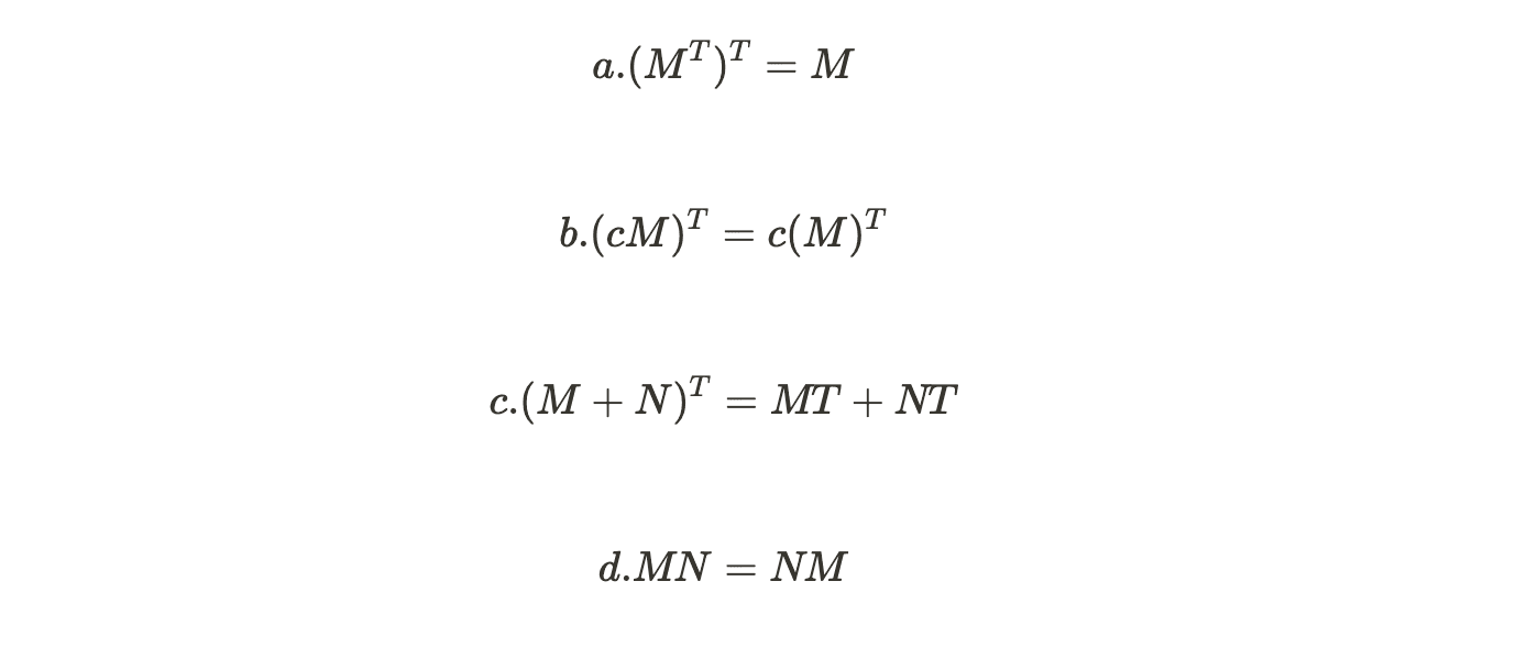
3. For matrices of same dimension M, N and scalar c, which one of these properties dose not always hold?

Solution:

d. MN = NM

4. Four matrices M1, M2, M3, and M4 have dimensions p x q, q x r, r x s, and s x t, respectively. They can be multiplied in different ways, resulting in different numbers of total scalar multiplications. If we multiply them as ((M1 x M2) x M3) x M4, the total number of scalar multiplications is pqr + pqrt. If we multiply them as (M1 x (M2 x M3)) x M4, the total number of scalar multiplications is pqrs + qrst. Given that p = 10, q = 100, r = 20, s = 5, and t = 80, what is the minimum number of scalar multiplications needed?

a. 248000

b. 44000

c. 19000

d. 25000

Solution:

c. 19000

Multiply as (M1 x M2) x M3) x M4 The total number of scalar multiplication is = qrs + pqs + pst =10000 + 5000 + 4000 = 19000

5. Given two vectors A = 3i + 4j and B = 5i - 2j, what is the magnitude of the vector sum A + B?

a. √10 b. √29 c. 7 d. 8

Solution:

b. √29

Explanation: To find the magnitude of the vector sum A + B, first add the two vectors:

A + B = (3i + 4j) + (5i - 2j) = 8i + 2j

Now, calculate the magnitude of the resulting vector:

|A + B| = √((8^2) + (2^2)) = √(64 + 4) = √68 = √(4 * 17) = 2√17

So, the magnitude of A + B is √29.