Probability Distributions for GATE Exam

In the context of the GATE (Graduate Aptitude Test in Engineering) exam, understanding probability distributions is pivotal. This introductory overview delves into the essential concepts and types of probability distributions, which play a crucial role in various engineering and science disciplines.

I. Introduction to Probability Theory

Definition of Probability:

Probability is a fundamental mathematical concept that quantifies uncertainty and measures the likelihood of various outcomes in a random experiment. It is a crucial tool used in a wide range of fields, from statistics to engineering, finance, physics, biology, and even machine learning.

Importance in Various Fields:

• Statistics: Probability plays a central role in statistics, allowing us to make inferences about populations based on sample data. It forms the foundation for statistical hypothesis testing and confidence intervals.
• Engineering: In engineering, probability is essential for reliability analysis. Engineers use probability to assess the likelihood of failure in systems and to design robust, dependable products.
• Finance: In finance, probability aids in risk management and investment strategies. It helps investors and financial institutions make informed decisions in uncertain markets.
• Physics: In physics, probability is a key element in quantum mechanics and statistical mechanics. It describes the behavior of particles at the quantum level and the statistical properties of macroscopic systems.
• Biology: Probability is used extensively in genetics, epidemiology, and evolutionary biology. It helps model genetic inheritance, disease spread, and evolutionary processes.
• Machine Learning: In machine learning, algorithms leverage probability to make predictions and classifications. Probability distributions are used to model uncertainties in data.

Basic Concepts:

Sample Space:

The sample space is the set of all possible outcomes of a random experiment. For example, when flipping a fair coin, the sample space consists of two outcomes: heads and tails.

Events:

Events are subsets of the sample space that represent specific outcomes or combinations of outcomes. Events can be simple (a single outcome) or compound (a combination of outcomes). For instance, "getting at least one head" when flipping a coin is a compound event.

Outcomes and Their Properties:

Outcomes are individual results within the sample space. Each outcome corresponds to a particular situation or observation. It's important to note that outcomes are mutually exclusive (only one can occur) and collectively exhaustive (at least one must occur).

Randomness and Uncertainty:

Randomness refers to the inherent unpredictability of certain events due to multiple factors or chance. Many real-world phenomena involve randomness, making precise predictions challenging. Probability theory helps us navigate this uncertainty by providing a formal framework for reasoning about randomness.

Uncertainty represents the degree of doubt or lack of precision associated with outcomes. Probability allows us to quantify and manage this uncertainty, aiding decision-making in the face of incomplete information.

Role of Probability Distributions:

Probability distributions are mathematical models that describe the likelihood of various outcomes in a random experiment. These distributions are central to probability theory as they enable us to:

• Predict future events based on historical data and patterns.
• Make informed decisions in uncertain situations.
• Perform statistical analysis, hypothesis testing, and risk assessment.

In the upcoming sections, we will delve deeper into different types of probability distributions, both discrete and continuous, and explore their applications in modeling real-world phenomena.

II. Discrete Probability Distributions

A. Discrete Random Variables

1. Definition of Random Variables:

Random variables are a fundamental concept in probability theory. They serve as a bridge between the outcomes of a random experiment and the mathematics of probability. A random variable is a numerical quantity whose value is determined by the outcome of a random experiment. It assigns a real number to each possible outcome in the sample space.

2. Role in Probability Theory:

Random variables are used to quantify and analyze uncertainty. They allow us to:

• Express the results of a random experiment in a mathematical form.
• Calculate probabilities associated with different outcomes.
• Formulate and solve problems involving uncertainty and randomness.

3. Discrete vs. Continuous Random Variables:

Discrete Random Variables are those that can take on a countable or finite number of distinct values. These values are typically separated by gaps and can be listed individually.

Continuous Random Variables, on the other hand, can take on an uncountable number of values within a given interval. They are characterized by a continuous probability distribution and can assume any value within a range.

4. Examples of Discrete Random Variables:

Example 1: Coin Toss

Consider the random variable X representing the number of heads obtained when flipping a fair coin three times. X can take on the values {0, 1, 2, 3}, representing the possible outcomes: 0 heads, 1 head, 2 heads, or 3 heads. Since these values are countable and distinct, X is a discrete random variable.

Example 2: Dice Roll

Suppose we roll a six-sided die, and Y represents the outcome. Y can take on the values {1, 2, 3, 4, 5, 6}, representing the possible outcomes of rolling a die. Like in the previous example, these values are countable and distinct, making Y a discrete random variable.

Example 3: Number of Defective Products

In a manufacturing process, Z represents the number of defective products in a batch of 100 items. Z can take on values {0, 1, 2, ..., 100}, representing the possible counts of defective products. Since there is a finite number of possible values (0 to 100), Z is a discrete random variable.

B. Probability Mass Function (PMF)

1. Definition of PMF:

The Probability Mass Function (PMF) is a fundamental concept in discrete probability distributions. It is a function that associates each possible value of a discrete random variable with its corresponding probability of occurrence. In essence, the PMF tells us how likely each outcome is.

2. Significance in Discrete Probability Distributions:

• Quantifying Probabilities: The PMF provides a systematic way to quantify the probabilities associated with each possible value of a discrete random variable.
• Summarizing Distribution: It summarizes the distribution of a discrete random variable, allowing us to understand its characteristics, such as the most likely values and the spread of probabilities.
• Basis for Calculations: The PMF forms the foundation for various calculations involving discrete random variables, including finding expected values, variances, and cumulative probabilities.

3. Properties of a Valid PMF:

A valid PMF must satisfy the following properties:

a. Non-Negativity:

• The probability for each possible value must be non-negative: P(_X_=x)≥0 for all x.

b. Sum of Probabilities:

• The sum of probabilities for all possible values must equal 1: ∑_P_(_X_=x)=1.

4. Calculating PMFs for Simple Random Variables:

Example 1: Coin Toss (Bernoulli Distribution)

Let's revisit the example of a fair coin toss where X represents the number of heads. The PMF for X is as follows:

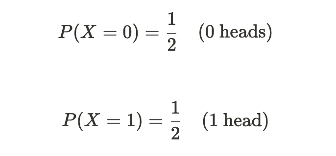
In this case, since there are only two possible outcomes (0 heads or 1 head), the PMF is straightforward.

Example 2: Dice Roll (Discrete Uniform Distribution)

Suppose Y represents the outcome of rolling a six-sided die. The PMF for Y is:

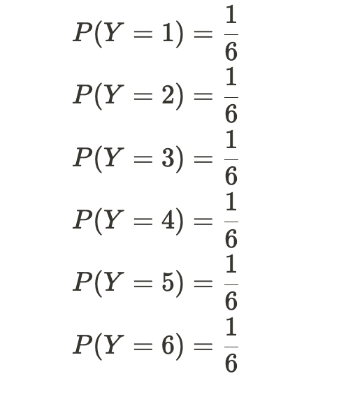
Here, all six outcomes are equally likely in a fair die, so each probability is 1/6.

Example 3: Number of Defective Products (Binomial Distribution)

Consider the random variable Z, representing the number of defective products in a batch of 100 items with a 5% defect rate. The PMF for Z follows the binomial distribution:

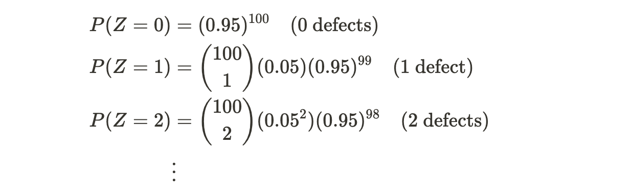
In this case, the PMF accounts for the probability of different numbers of defects in a batch.

C. Common Discrete Probability Distributions

1. Uniform Distribution:

Explanation:

The Uniform Distribution is a discrete probability distribution where all possible outcomes are equally likely. It is often used when each outcome has the same chance of occurring.

Real-World Examples and Use Cases:

Rolling a Fair Die: The outcome of rolling a fair six-sided die follows a uniform distribution, where each number (1 to 6) has an equal probability of 61.

16

Calculation:

To calculate probabilities:

• For a discrete uniform distribution with n equally likely outcomes, the probability of any specific outcome is

To calculate the expected value (mean):

• The expected value for a uniform distribution with outcomes a to b is

2. Bernoulli Distribution:

Explanation:

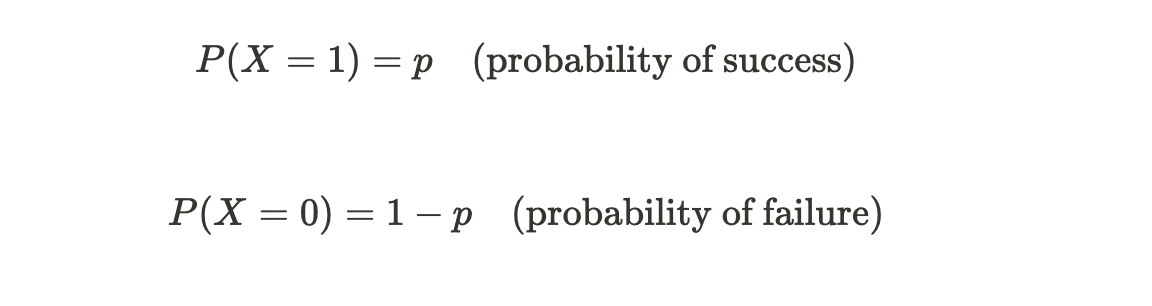
The Bernoulli Distribution models a binary experiment with two possible outcomes: success (usually denoted as 1) and failure (usually denoted as 0). It is often used for situations with only two possible results.

Real-World Examples and Use Cases:

• Coin Flip: Modeling the outcome of a fair coin toss, where success might represent "heads" (1) and failure represents "tails" (0).
• Email Delivery: Modeling whether an email gets delivered (success) or bounces (failure).

Calculation:

To calculate probabilities:

To calculate the expected value (mean):

• The expected value for a Bernoulli distribution with probability p of success is

3. Binomial Distribution:

Explanation:

The Binomial Distribution models a sequence of independent Bernoulli trials, where each trial results in a binary outcome (success or failure). It calculates the probability of achieving a specific number of successes in a fixed number of trials.

Real-World Examples and Use Cases:

• Quality Control: Calculating the probability of a certain number of defective products in a batch.
• Survey Responses: Estimating the likelihood of getting a certain number of "yes" responses in a survey.

Calculation:

To calculate probabilities:

• where k is the number of successes, n is the number of trials, and p is the probability of success in a single trial.

To calculate the expected value (mean):

• The expected value for a binomial distribution with parameters n (number of trials) and p (probability of success in a single trial) is

4. Poisson Distribution:

Explanation:

The Poisson Distribution models the number of events that occur in a fixed interval of time or space. It's often used to describe rare events that happen with a known average rate.

Real-World Examples and Use Cases:

• Call Center Incoming Calls: Modeling the number of calls received in a minute.
• Accident Reporting: Estimating the number of accidents at a particular intersection in a day.

Calculation:

To calculate probabilities:

• where k is the number of events, and λ is the average rate of events in the given interval.

To calculate the expected value (mean):

• The expected value for a Poisson distribution with rate λ is

These distributions are essential tools for modeling and analyzing various real-world phenomena, allowing us to make informed decisions and predictions based on probability theory.

III. Continuous Probability Distributions

A. Continuous Random Variables

1. Definition of Continuous Random Variables:

Continuous random variables are variables that can take on any real value within a specified range or interval. Unlike discrete random variables, which have distinct, countable outcomes, continuous random variables can assume an uncountable number of values within their domain. They are often used to model measurements or quantities that can vary continuously.

2. Characteristics of Continuous Random Variables:

• Uncountable Outcomes: Continuous random variables can take on an infinite number of possible values within a given interval.
• Probability Density: Instead of assigning probabilities to individual outcomes, continuous random variables are described using probability density functions (PDFs).
• No Point Probabilities: The probability of a continuous random variable taking on a specific value is typically zero due to the infinite number of possible values.

3. Probability Density Function (PDF):

The Probability Density Function (PDF) is a function that describes the probability distribution of a continuous random variable. It indicates how the probability is distributed across the range of possible values. The PDF is characterized by the following properties:

• It is non-negative: f(x)≥0 for all x.
• The total area under the PDF curve over its entire range is equal to 1

• The probability of a continuous random variable falling within a specific interval is given by the integral of the PDF over that interval.

4. Examples of Continuous Random Variables:

Example 1: Height of Adults

The height of adults is a continuous random variable because it can vary continuously between certain minimum and maximum values. A PDF can describe the distribution of adult heights in a population.

Example 2: Temperature

Temperature is another continuous random variable. It can take on any value within a given range (e.g., -273.15°C to positive infinity). A PDF can represent the distribution of temperatures.

Example 3: Time to Failure

In reliability engineering, the time until a component or system fails is modeled as a continuous random variable. A PDF can describe the probability of failure at various time points.

B. Probability Density Function (PDF)

1. Definition of PDF and Its Properties:

Probability Density Function (PDF) is a fundamental concept in continuous probability distributions. It's a function that describes the likelihood of a continuous random variable taking on a specific value within a given interval. Key properties of PDFs include:

• Non-Negativity: The PDF is non-negative for all values of the random variable: f(x)≥0.
• Area under the Curve: The total area under the PDF curve over its entire range is equal to 1:

• Probability Interpretation: The probability of a random variable falling within a specific interval is given by the integral of the PDF over that interval.

2. Comparison of PMFs and PDFs:

Probability Mass Functions (PMFs) are used for discrete random variables and provide the probability of specific values. In contrast, PDFs are used for continuous random variables and give probabilities for ranges of values. PMFs assign probabilities to individual outcomes, while PDFs provide probabilities for intervals.

3. Calculating Probabilities and Expected Values with PDFs:

Probability Calculation:

To find the probability that a continuous random variable X falls within an interval [a,_b_], you can use the integral of the PDF over that interval:

This integral represents the probability that X falls between a and b.

Expected Value Calculation:

The expected value (mean) of a continuous random variable X with PDF f(x) is calculated as:

This integral represents the weighted average of all possible values of X.

Example: Calculating Probabilities and Expected Values with a PDF

Problem:

Suppose we have a continuous random variable X with the following PDF:

a) Find the probability that X falls between 0.2 and 0.5.

b) Calculate the expected value (μ) of X.

Solution:

a) To find the probability that X falls between 0.2 and 0.5, we need to calculate the integral of the PDF f(x) over the interval [0.2 , 0.5]:

Now, calculate the integral:

So, the probability that X falls between 0.2 and 0.5 is 0.21.

b) To calculate the expected value (μ) of X, we use the following formula:

Plug in the PDF f(x):

Calculate the integral:

So, the expected value (μ) of X is 2/3.

Answers:

a) The probability that X falls between 0.2 and 0.5 is 0.21.

b) The expected value (μ) of X is 2/3.

C. Common Continuous Probability Distributions

1. Normal Distribution:

• Definition: The Normal Distribution, also known as the Gaussian distribution, is a symmetric bell-shaped distribution characterized by its mean (μ) and standard deviation (σ). The probability density function (PDF) of the normal distribution is given by:

• Real-World Applications: The normal distribution is commonly found in nature and various human characteristics, such as height, IQ scores, and measurement errors. It's also used in finance, engineering, and quality control.
• Calculations: To calculate probabilities and expected values, you can use standard tables, statistical software, or calculus-based integration.

2. Exponential Distribution:

• Definition: The Exponential Distribution models the time between events in a Poisson process. It's characterized by the rate parameter (λ). The PDF of the exponential distribution is given by:

• Real-World Applications: It's used to model waiting times, such as the time between customer arrivals at a service center, the lifespan of electronic components, and the time between arrivals of buses at a bus stop.
• Calculations: Probabilities and expected values are calculated using integration techniques.

3. Uniform Distribution (Continuous Version):

• Definition: The Uniform Distribution describes a continuous random variable where all values within a specified range are equally likely. The PDF of the uniform distribution is constant within the range [a,_b_] and zero outside this range.
• Real-World Applications: It's used in scenarios where all outcomes are equally probable, such as modeling the randomness in lottery numbers or the arrival time of customers at a store when they are uniformly distributed.
• Calculations: Calculating probabilities is straightforward because the PDF is constant over the range, and expected values are found using the mean of the uniform distribution.

4. Gamma Distribution:

• Definition: The Gamma Distribution is a flexible distribution characterized by two parameters: shape (k) and scale (θ). The PDF of the gamma distribution is given by:

• Real-World Applications: It's used to model waiting times, insurance claims, and the distribution of income. It's also relevant in reliability analysis.
• Calculations: Probabilities and expected values require integration techniques, and the gamma function Γ(k) may need to be computed.

These common continuous probability distributions are fundamental tools in statistics and have numerous applications across various fields. Understanding their properties and how to calculate probabilities and expected values is essential for data analysis and modeling.

Conclusion

Probability theory is a foundational concept with broad applications across various fields, including statistics, engineering, finance, and biology. It helps quantify uncertainty and make informed decisions in the face of randomness. Understanding both discrete and continuous probability distributions is essential for modeling and analyzing real-world phenomena.

Key Takeaways

1. Probability's Ubiquity: Probability theory is essential in diverse fields, from statistics to finance, where it's used to make predictions and manage risk.
2. Discrete vs. Continuous: Random variables can be discrete (countable outcomes) or continuous (uncountable outcomes within an interval), each requiring different probability models.
3. PMFs and PDFs: Discrete random variables use Probability Mass Functions (PMFs) to assign probabilities to values, while continuous random variables use Probability Density Functions (PDFs) for intervals.
4. Common Distributions: Understanding common probability distributions like the normal, exponential, uniform, and gamma distributions is crucial for solving real-world problems and calculating probabilities and expected values.

Practice Questions:

1. A probability density function on the interval [a, 1] is given by 1 / x^2 and outside this interval the value of the function is zero. The value of a is :

(A) -1

(B) 0

(C) 1

(D) 0.5

Answer:

(D)

Explanation:

But, this is equal to 1.

So, (-1) + (1/a) = 1

Therefore, a = 0.5

2. Suppose Xi for i = 1, 2, 3 are independent and identically distributed random variables whose probability mass functions are Pr[Xi = 0] = Pr[Xi = 1] = 1/2 for i = 1, 2, 3. Define another random variable Y = X1 X2 ⊕ X3, where ⊕ denotes XOR.

Then Pr[Y = 0 ⎪ X3 = 0] = ____________.

(A) 0.75

(B) 0.50

(C) 0.85

(D) 0.25

Answer:

(A)

Explanation:

P (A|B) = P (A∩B) / P (B)

P (Y=0 | X3=0) = P(Y=0 ∩X3=0) / P(X3=0)

P(X3=0) = 1⁄2

Y = X1X2 ⊕ X3

From the above table, P(Y=0 ∩X3=0) = 3/8And P (X3=0) = 1⁄2

P (Y=0 | X3=0) = P(Y=0 ∩X3=0) / P(X3=0) = (3/8) / (1/2) = 3⁄4 = 0.75

This solution is contributed by Anil Saikrishna Devarasetty .

Another Solution :

It is given X3 = 0.

Y can only be 0 when X1 X2 is 0. X1 X2 become 0 for X1 = 1, X2 = 0, X1 = X2 = 0 and X1 = 0, X = 1

So the probability is = 0.5_0.5_3 = 0.75

3. Consider a quiz where a person is given two questions and he must decide which question to answer first. Question 1 will be answered correctly with probability of 0.8 and the person will then receive as prize $100, while question 2 will be answered correctly with probability 0.5, and the person will then receive as prize $200. If the first question is answered incorrectly then the quiz terminates and that person is not allowed to attempt the second question. What is the expected amount of money that can he win?

Answer:

Let's define some variables:

• Let X be the random variable representing the amount of money the person wins.
• Let A be the event that the person chooses to answer Question 1.
• Let B be the event that the person answers Question 1 correctly.
• Let C be the event that the person answers Question 2 correctly.
• P(A) = Probability of choosing Question 1 = 1/2 (since the person has two questions to choose from).
• P(B|A) = Probability of answering Question 1 correctly given that Question 1 is chosen = 0.8.
• P(C|B) = Probability of answering Question 2 correctly given that Question 1 is answered correctly = 0.5.

1. If the person chooses to answer Question 1 (event A):
   • If the person answers it correctly (event B), they win $100.
   • If the person answers it incorrectly (event B' or not B), the quiz terminates, and they win $0.
   • So, E(X|A) = $100 * P(B|A) + $0 * P(B'|A) = $100 * 0.8 + $0 * 0.2 = $80.
2. If the person chooses not to answer Question 1 (event A' or not A):
   • The quiz terminates, and they win $0.
   • So, E(X|A') = $0.

4. Let X be a discrete random variable. The probability distribution of X is given below:

Then E(X) is equal to a. 6 b. 4 c. 3 d. −5

Answer:

To calculate the expected value (E(X)) of a discrete random variable X, you need to multiply each possible value of X by its corresponding probability and then sum them up. Here's how you can calculate E(X) based on the provided probability distribution:

E(X) = (X₁ * P(X₁)) + (X₂ * P(X₂)) + (X₃ * P(X₃))

Where:

• X₁ is the first possible value of X (30).
• X₂ is the second possible value of X (10).
• X₃ is the third possible value of X (-10).
• P(X₁) is the probability of X being equal to X₁ (1/5).
• P(X₂) is the probability of X being equal to X₂ (3/10).
• P(X₃) is the probability of X being equal to X₃ (1/2).

5. The lifetime of a component of a certain type is a random variable whose probability density function is exponentially distributed with parameter 2. For a randomly picked component of this type, the probability that its lifetime exceeds the expected lifetime (rounded to 2 decimal places) is ____________.

Answer:

The probability that the lifetime of a component exceeds its expected lifetime can be found using the properties of the exponential distribution. In this case, we are given that the lifetime follows an exponential distribution with a parameter λ (which is also the reciprocal of the expected lifetime).

Let's denote the expected lifetime as E(X). It is known that for an exponential distribution:

E(X) = 1 / λ

We are interested in finding the probability that the lifetime exceeds the expected lifetime:

P(X > E(X))

Substitute E(X) with 1/λ:

P(X > 1/λ)

Now, let's integrate the exponential probability density function from E(X) to infinity to find this probability:

P(X > 1/λ) = ∫[1/λ, ∞] λ * e^(-λx) dx

Integrate from 1/λ to ∞:

P(X > 1/λ) = -e^(-λx) | from 1/λ to ∞

P(X > 1/λ) = (-e^(-∞λ)) - (-e^(-1))

As λ approaches infinity, e^(-∞λ) approaches 0, so the first term becomes 0:

P(X > 1/λ) = 0 - (-e^(-1))

P(X > 1/λ) = e^(-1)

Now, calculate the value of e^(-1):

e^(-1) ≈ 0.36788 (rounded to five decimal places)

So, the probability that the lifetime of a randomly picked component exceeds its expected lifetime is approximately 0.36788 when rounded to the required number of decimal places.