Reasoning under Uncertainty for GATE Exam

Uncertainty refers to a lack of complete knowledge or predictability about a future event or outcome. In decision-making, uncertainty is a critical concept because it reflects the degree of doubt or ambiguity surrounding potential outcomes. Uncertainty can arise from various sources, including incomplete information, randomness, or the inherent complexity of a situation. Its significance in decision-making lies in the fact that it directly impacts the quality and rationality of decisions. Decision-makers must account for uncertainty when making choices because failing to do so can lead to poor decisions, unexpected consequences, and increased risk.

Probability as a Measure of Uncertainty

Probability is a mathematical concept used to quantify uncertainty. It provides a way to express and quantify the likelihood of different outcomes in uncertain situations. In decision-making, probability serves as a measure of how likely or unlikely a particular event or outcome is to occur. By assigning probabilities to different scenarios, decision-makers can make more informed choices and assess the potential risks associated with their decisions.

Probability theory and random variables form the foundation for quantifying and managing uncertainty in decision-making processes, allowing decision-makers to make informed choices while acknowledging the inherent unpredictability of many real-world situations.

Bayesian Networks

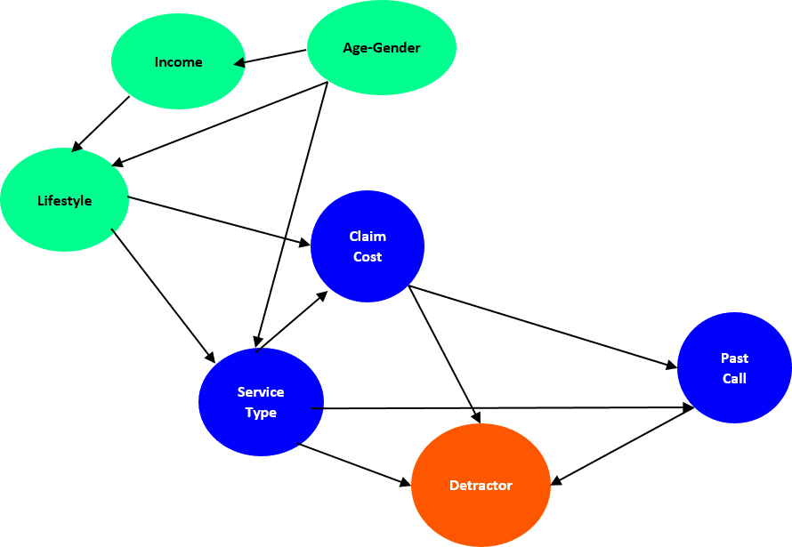
Bayesian Network

Bayesian networks, also known as belief networks or Bayes networks, are graphical models used to represent and reason about uncertain knowledge and probabilistic relationships between variables. They are named after the Reverend Thomas Bayes and provide a structured way to model and analyze complex systems by capturing dependencies and uncertainties among variables. Bayesian networks are widely used in fields such as artificial intelligence, machine learning, medicine, and decision support systems.

Nodes, Edges, and Conditional Probability Tables (CPTs) in Bayesian Networks:

• Nodes: In a Bayesian network, nodes represent random variables or variables of interest. Each node corresponds to a specific variable or event in the domain being modeled. Nodes can be categorized into two types:
  • Chance Nodes (or Random Variables): These nodes represent uncertain variables that can take on different values. For example, in a medical diagnosis Bayesian network, a chance node might represent the presence or absence of a disease.
  • Decision Nodes (or Control Variables): These nodes represent variables under the control of the decision-maker, such as treatment options in a medical decision-making context.
• Edges: Edges in a Bayesian network represent probabilistic dependencies between nodes. An edge from Node A to Node B indicates that Node B's probability distribution depends on Node A. This directional relationship signifies that Node A is a parent of Node B, and Node B is a child of Node A.
• Conditional Probability Tables (CPTs): CPTs are associated with each chance node in the Bayesian network. They specify the conditional probabilities of a node taking on a particular value given the values of its parent nodes. CPTs quantify the probabilistic relationships between variables. For example, if a disease node has two parent nodes representing symptoms, the CPT for the disease node would specify the probability of the disease given the observed symptoms.

Performing Inference in Bayesian Networks

Inference in Bayesian networks involves using the network structure and CPTs to compute probabilities of interest or make predictions. Two common types of inference in Bayesian networks are:

• Marginal Inference: This involves calculating the probability distribution of one or more variables of interest without specifying the values of other variables. It's often used to answer questions like "What is the probability of disease D given the observed symptoms?"
• Conditional Inference: In this type of inference, some variables are observed (given specific values), and the goal is to calculate the probability distribution of other variables conditional on the observed values. For instance, "Given that a patient has a certain symptom, what is the probability of having a particular disease?"

Bayesian networks use the principles of probability theory, including Bayes' theorem, to perform inference. The steps for inference typically involve:

a. Propagation: This step involves propagating information through the network to update the beliefs about variables based on the evidence (observed values).

b. Normalization: After propagation, the probabilities are often normalized to ensure that they sum up to 1.

c. Querying: Once the network is updated with evidence and probabilities are normalized, you can query the network to obtain answers to specific probabilistic questions.

Bayesian networks are particularly useful for handling uncertainty in complex systems, and their graphical representation makes them intuitive for modeling and decision-making in various domains. They enable decision-makers to make informed choices based on probabilistic reasoning and available evidence.

Exact Inference in Bayesian Networks

Exact inference methods in Bayesian networks are techniques for calculating the exact probabilities of variables of interest given the network structure and evidence (observed variable values). Two common methods for exact inference in Bayesian networks are Variable Elimination and the Junction Tree algorithm.

1. Variable Elimination:
   • Principle: Variable Elimination is a systematic method for computing marginal probabilities of variables in a Bayesian network. It works by iteratively eliminating variables from the network, simplifying the computation until the desired probabilities are obtained.
   • Steps:
     1. Initialize: Begin with the full Bayesian network.
     2. Enter Evidence: Set observed variables to their observed values, reducing the problem's scope.
     3. Variable Elimination: Eliminate non-query variables one at a time by summing over their values while considering conditional probabilities.
     4. Repeat step 3 until only the query variable(s) remain.
     5. Calculate Final Probability: Compute the desired probability based on the remaining factors.
2. Junction Tree Algorithm:
   • Principle: The Junction Tree algorithm is an advanced method for exact inference in Bayesian networks. It transforms the original Bayesian network into a tree-like structure (junction tree or clique tree), where inference becomes more efficient. It uses the concept of message-passing to propagate beliefs and calculate probabilities.
   • Steps:
     1. Construct a Junction Tree: Transform the Bayesian network into a Junction Tree by identifying clusters of variables (cliques) and creating a tree structure connecting them.
     2. Enter Evidence: Set observed variables to their observed values, reducing the problem's scope.
     3. Message Passing: Perform message-passing operations (belief propagation) within the tree structure to calculate the joint probability distribution over all variables.
     4. Calculate Marginal Probabilities: Once the joint distribution is obtained, marginal probabilities for query variables can be calculated efficiently.

Principles of Exact Inference in Bayesian Networks

The principles of exact inference in Bayesian networks revolve around using probabilistic reasoning and the network's structure to compute probabilities accurately. Key principles include:

1. Conditional Probability: Exact inference relies on conditional probabilities specified in the Conditional Probability Tables (CPTs) of the network. These tables express the probabilistic relationships between variables in the network.
2. Evidence Propagation: When evidence is entered (observed variable values), the inference process involves propagating this evidence through the network to update beliefs about other variables.
3. Variable Elimination: In variable elimination, non-query variables are systematically eliminated from consideration, simplifying the computation while preserving the correctness of the results.
4. Tree Structure (Junction Tree): The Junction Tree algorithm transforms the network into a tree structure, which ensures that messages passed between variables converge to a unique solution. This tree structure is crucial for efficient inference.

Examples of Exact Inference in Practical Problems:

1. Medical Diagnosis: Bayesian networks are used in medical diagnosis. For instance, a network might model symptoms, diseases, and test results. Exact inference can determine the probability of a specific disease given observed symptoms and test outcomes.
2. Natural Language Processing: In language processing, Bayesian networks can represent the relationships between words, grammar rules, and meanings. Exact inference can help determine the most likely interpretation of a sentence given observed words.
3. Fraud Detection: In financial systems, Bayesian networks can model transactions, account behavior, and fraud indicators. Exact inference can identify the likelihood of a transaction being fraudulent based on observed patterns.
4. Robotics and Autonomous Vehicles: Bayesian networks are used for decision-making in robotics and autonomous vehicles. Inference can help these systems reason about sensor data to make safe and efficient decisions, such as path planning.

Exact inference methods ensure that probabilities are computed rigorously in Bayesian networks, making them valuable tools for various applications where uncertainty and probabilistic reasoning play a crucial role in decision-making.

Approximate Inference in Bayesian Networks

Approximate inference methods are techniques used in Bayesian networks to estimate probabilities or make decisions when exact inference is computationally infeasible or impractical due to the complexity of the network. Two common approximate inference methods are Markov Chain Monte Carlo (MCMC) and belief propagation.

1. Markov Chain Monte Carlo (MCMC):
   • MCMC is a probabilistic sampling technique used to approximate the posterior distribution of variables in a Bayesian network. It's particularly useful when dealing with high-dimensional and complex probability distributions.
   • In MCMC, a Markov chain is constructed, where each state of the chain represents a possible configuration of variables. The chain is sampled over a large number of iterations, and the samples converge to an approximation of the true posterior distribution.
   • Common MCMC algorithms include Metropolis-Hastings and Gibbs sampling.
2. Belief Propagation:
   • Belief propagation is an approximate inference algorithm mainly used in graphical models such as Bayesian networks and factor graphs.
   • It operates on the principle of message-passing, where nodes exchange messages with their neighboring nodes to iteratively update beliefs about the variables. Belief propagation can be used for marginalization and maximum a posteriori (MAP) estimation.
   • However, belief propagation is exact only for trees and can introduce approximation errors in more complex network structures.

Trade-offs Between Exact and Approximate Inference

1. Computational Complexity:
   • Exact inference methods guarantee precise results but can be computationally expensive, especially for large and complex networks. Approximate methods like MCMC and belief propagation are often faster and more scalable.
2. Accuracy:
   • Exact inference methods provide accurate results, but they may not be feasible in practice for networks with a large number of variables or complex dependencies. Approximate methods sacrifice some accuracy for computational efficiency.
3. Convergence:
   • Exact inference methods always converge to the correct solution given enough computation time. Approximate methods might not guarantee convergence to the true solution but offer reasonable approximations within a specified time frame.
4. Applicability:
   • Exact inference is typically used when precision is critical, or when the network is small enough to handle exact calculations. Approximate inference is essential for handling large, complex networks or when real-time decision-making is required.

Use of Approximate Inference in Large and Complex Networks

Approximate inference is particularly valuable in large and complex Bayesian networks for the following reasons:

1. Scalability: Exact inference becomes impractical when dealing with a large number of variables or intricate dependencies. Approximate methods like MCMC can provide reasonably accurate results in such scenarios.
2. Real-Time Decision-Making: In applications like robotics, finance, and healthcare, decisions often need to be made quickly. Approximate methods allow for rapid inference, making them suitable for time-sensitive tasks.
3. Resource Constraints: In resource-constrained environments, such as edge devices or low-power hardware, approximate inference may be the only viable option due to limited computational resources.
4. Exploration of High-Dimensional Spaces: MCMC, in particular, is useful for exploring high-dimensional probability spaces, which is often required in machine learning and statistical modeling.
5. Handling Loopy Networks: Bayesian networks with loops can be problematic for exact inference methods. Belief propagation, while approximate, can be applied to such networks to provide useful approximations.

In summary, approximate inference methods strike a balance between computational efficiency and accuracy, making them indispensable in scenarios where exact inference is not feasible or where timely decision-making is crucial. They are particularly valuable in large and complex Bayesian networks and have a wide range of applications in various fields.

Decision Making under Uncertainty

Decision-making in uncertain environments involves making choices when outcomes are not entirely predictable. It's a fundamental aspect of both everyday life and various fields like business, finance, healthcare, and artificial intelligence. Uncertainty arises due to incomplete information, randomness, or the complexity of the environment. To make informed decisions in such situations, various approaches and tools are employed.

Decision Making under Uncertainty

Introduction to Decision Trees

Decision trees are a graphical representation of decision-making processes. They are used to model decisions and their potential consequences in a structured way, making them particularly valuable in uncertain environments. Decision trees consist of nodes and branches and are commonly used in conjunction with utility theory, a framework for quantifying preferences.

1. Nodes:
   • Decision Nodes: Represent choices or decisions that need to be made. They have branches leading to different possible actions.
   • Chance Nodes (or Probability Nodes): Represent uncertain events or states of nature. They have branches leading to possible outcomes.
   • Terminal Nodes (or Utility Nodes): Represent the final outcomes of a decision process and include a value representing the utility or desirability of that outcome.
2. Branches:
   • Branches connect nodes and represent the different possible paths or choices in the decision-making process.

Utility Theory:

Utility theory is a framework for quantifying preferences and decision-making under uncertainty. It involves assigning numerical values called utilities to different outcomes or states of nature to express a decision-maker's preferences. The key principles of utility theory include:

1. Utility Functions: These functions map outcomes or states to utility values. They reflect a decision-maker's preferences and quantify the desirability of different outcomes.
2. Expected Utility: Expected utility is a concept that combines the utility values and the probabilities associated with different outcomes. It calculates the average utility a decision-maker can expect to receive for a particular decision.

Making Decisions Using Probabilistic Reasoning:

To make decisions using probabilistic reasoning, you can follow these steps:

1. Define the Decision Problem: Clearly specify the decision to be made and identify all relevant variables, including decision nodes, chance nodes, and utility nodes.
2. Construct the Decision Tree: Create a decision tree that represents the decision problem. Use decision nodes to denote choices, chance nodes to denote uncertain events, and terminal nodes to assign utility values to outcomes.
3. Assign Probabilities and Utilities: Assign probabilities to the branches emanating from chance nodes, reflecting the likelihood of each outcome. Additionally, assign utility values to terminal nodes to represent preferences.
4. Calculate Expected Utilities: Calculate the expected utilities for each decision alternative by multiplying the utilities by their respective probabilities and summing them up along each path through the decision tree.
5. Make the Decision: Choose the decision alternative with the highest expected utility. This is known as the "maximize expected utility" criterion and is a rational choice under uncertainty.
6. Sensitivity Analysis: Assess the robustness of your decision by varying the probabilities and utilities to understand how changes might impact the chosen decision.

Probabilistic reasoning, decision trees, and utility theory provide a structured framework for making decisions in uncertain environments. By quantifying probabilities and preferences, decision-makers can systematically evaluate their options and choose the best course of action based on their objectives and the available information.

Fuzzy Logic

Fuzzy logic is a mathematical framework and a form of multi-valued logic that is designed to handle uncertainty and vagueness in a more flexible and human-like manner. Unlike classical binary logic, which relies on strict true or false values, fuzzy logic allows for degrees of truth between 0 and 1, making it suitable for modeling and reasoning in situations where information is imprecise or uncertain.

Components of Fuzzy Logic:

1. Fuzzy Sets:
   • Fuzzy sets are a fundamental concept in fuzzy logic. Unlike traditional sets, where an element is either a member (1) or not a member (0), fuzzy sets allow for gradual or partial membership. Each element belongs to a fuzzy set with a degree of membership between 0 and 1, indicating the strength of membership.
2. Membership Functions:
   • Membership functions define the shape and characteristics of a fuzzy set. They map each element's value to its degree of membership in the set. Membership functions can take various forms, such as triangular, trapezoidal, Gaussian, or sigmoidal, depending on the specific problem domain.
3. Fuzzy Rules:
   • Fuzzy rules are logical expressions that describe relationships between fuzzy sets. They consist of antecedents (if-conditions) and consequents (then-actions). Fuzzy rules use linguistic variables and fuzzy logic operators (AND, OR, NOT) to represent imprecise knowledge and reasoning.

Applications of Fuzzy Logic in AI and Decision-Making:

Fuzzy logic finds numerous applications in various fields, including artificial intelligence, control systems, and decision-making, due to its ability to handle uncertainty and vagueness effectively. Some notable applications include:

1. Fuzzy Control Systems:
   • Fuzzy logic is extensively used in control systems, especially in situations where precise mathematical models are unavailable or too complex. Fuzzy control allows for real-time decision-making in systems like automotive ABS (anti-lock braking systems), HVAC (heating, ventilation, and air conditioning), and industrial processes.
2. Pattern Recognition:
   • Fuzzy logic can be applied in pattern recognition tasks, such as image and speech recognition, where objects or patterns may have ambiguous or overlapping features.
3. Natural Language Processing:
   • Fuzzy logic is valuable in natural language processing for handling the inherent vagueness and ambiguity in human language. It can be used for tasks like sentiment analysis, text summarization, and information retrieval.
4. Medical Diagnosis:
   • Fuzzy logic aids medical experts in diagnosing diseases and conditions where symptoms and test results are imprecise. Fuzzy systems can provide probabilistic diagnoses based on degrees of symptom severity.
5. Traffic Control:
   • Fuzzy logic is employed in traffic signal control systems to optimize traffic flow at intersections. It considers factors like traffic volume, vehicle speed, and pedestrian activity to adjust signal timings dynamically.
6. Decision Support Systems:
   • In decision support systems, fuzzy logic can be used to model decision-making processes when dealing with imprecise or qualitative information. It helps decision-makers consider multiple criteria and preferences.
7. Consumer Electronics:
   • Fuzzy logic is used in consumer products like washing machines to automatically adjust washing parameters based on the type and quantity of laundry, achieving better energy efficiency and washing performance.

Fuzzy logic's ability to capture and model uncertainty and vagueness makes it a powerful tool for addressing real-world problems where conventional crisp logic and numerical methods may fall short. It enables systems to make more human-like, nuanced decisions, which is especially valuable in complex and uncertain environments.

Uncertainty in Machine Learning

Uncertainty is a critical aspect of machine learning, and various techniques are used to address it in different types of models. Here are some approaches for handling uncertainty in machine learning models:

1. Probabilistic Models:
   • Probabilistic models explicitly model uncertainty by providing probability distributions over outcomes. Examples include Gaussian Mixture Models (GMMs) and Hidden Markov Models (HMMs).
   • In regression tasks, Bayesian Linear Regression provides not only point estimates of predictions but also uncertainty estimates in the form of posterior distributions.
2. Bayesian Neural Networks (BNNs):
   • Bayesian Neural Networks extend traditional neural networks by treating weights as probability distributions rather than fixed values. This allows them to capture model uncertainty.
   • BNNs provide predictive uncertainty in classification and regression tasks, which can be beneficial for decision-making.
3. Ensemble Methods:
   • Ensemble methods like Random Forests and Gradient Boosting construct multiple models and combine their predictions. They can provide uncertainty estimates by assessing the variability in predictions across ensemble members.
4. Monte Carlo Dropout:
   • Applying dropout during both training and inference in deep neural networks with Monte Carlo sampling can produce approximate posterior predictive distributions, enabling uncertainty estimation.
5. Uncertainty Quantification Techniques:
   • Techniques like bootstrapping, cross-validation, and jackknife resampling help quantify uncertainty by assessing how model performance varies with different subsets of the data.

How Uncertainty Quantification Improves Model Reliability:

Uncertainty quantification enhances model reliability and decision-making in several ways:

1. Risk Assessment:
   • Understanding uncertainty allows decision-makers to assess the potential risks associated with model predictions. They can make more informed decisions when they know the level of uncertainty in the model's output.
2. Robustness:
   • Models that provide uncertainty estimates are more robust in situations where the data distribution changes or when data is noisy. Decision-makers can adapt their strategies based on the confidence level of predictions.
3. Decision Thresholds:
   • Uncertainty quantification helps set decision thresholds. In critical applications like medical diagnosis, a higher level of uncertainty may lead to additional tests or a more conservative approach.
4. Resource Allocation:
   • Knowing uncertainty allows for better resource allocation. For example, in supply chain management, understanding demand uncertainty can help optimize inventory levels and production schedules.
5. Trust and Accountability:
   • Models that provide uncertainty estimates are more transparent and trustworthy. They allow stakeholders to assess model reliability and understand when caution is needed.

Examples of Machine Learning Applications Involving Uncertainty:

1. Self-Driving Cars:
   • Autonomous vehicles use probabilistic models and Bayesian techniques to estimate uncertainty in sensor data, allowing them to make safe decisions, especially in adverse weather conditions or complex traffic scenarios.
2. Medical Diagnostics:
   • Medical image analysis often involves uncertainty quantification to assess the confidence of diagnostic predictions. Radiologists can make more informed decisions based on the level of uncertainty.
3. Financial Forecasting:
   • In financial markets, models that provide uncertainty estimates help investors manage risk, make trading decisions, and optimize portfolio allocation.
4. Natural Language Processing:
   • In sentiment analysis, understanding the uncertainty in sentiment predictions is crucial for generating more reliable sentiment scores and summaries.
5. Manufacturing Quality Control:
   • Uncertainty quantification is used in quality control to assess the reliability of product specifications and detect defects or anomalies in manufacturing processes.
6. Environmental Monitoring:
   • In climate modeling, uncertainty quantification helps policymakers make decisions based on probabilistic predictions of future climate conditions.

In these and many other applications, addressing uncertainty in machine learning models improves their practical utility, reliability, and effectiveness in decision-making processes.

Conclusion

In this lesson, we explored the critical concept of uncertainty and its profound impact on decision-making processes. We discussed how uncertainty can arise from various sources, emphasizing its significance in decision-making. Probability theory, random variables, and Bayesian networks were introduced as fundamental tools for modeling and quantifying uncertainty. We delved into both exact and approximate inference methods in Bayesian networks, showcasing their applications in handling uncertainty effectively.

Furthermore, we discussed decision-making frameworks, including decision trees, utility theory, and fuzzy logic, which provide structured approaches to making choices in uncertain environments. We examined how these frameworks facilitate probabilistic reasoning, enabling decision-makers to navigate complex and ambiguous situations.

Key Takeaways:

• Uncertainty is the lack of complete knowledge or predictability about future events or outcomes, impacting decision-making quality and rationality.
• Probability serves as a measure of uncertainty, quantifying the likelihood of different outcomes in uncertain situations.
• Bayesian networks are graphical models that represent and reason about uncertain knowledge, using nodes, edges, and conditional probability tables (CPTs).
• Exact inference methods, such as variable elimination and the junction tree algorithm, provide precise solutions but can be computationally intensive.
• Approximate inference methods, like Markov Chain Monte Carlo (MCMC) and belief propagation, offer more scalable solutions for complex networks.
• Decision trees, utility theory, and fuzzy logic provide structured frameworks for decision-making in uncertain environments.
• Fuzzy logic handles uncertainty by allowing for gradual or partial membership in fuzzy sets, enhancing decision-making in various applications.
• Uncertainty quantification improves model reliability, aids risk assessment, and supports better resource allocation in decision-making processes.
• Machine learning applications involving uncertainty range from self-driving cars and medical diagnostics to financial forecasting and environmental monitoring, where understanding and managing uncertainty are critical for success.

Practice Questions

1. What does the concept of "uncertainty" refer to in decision-making?

A. The complete knowledge about future events. 

B. The predictability of future events. 

C. The degree of doubt or ambiguity surrounding potential outcomes. 

D. The complexity of decision-making.

Answer:

C. The degree of doubt or ambiguity surrounding potential outcomes.

2. In Bayesian networks, what do nodes represent?

A. Decision alternatives. 

B. Uncertain events. 

C. The complexity of the problem. 

D. Probability distributions.

Answer:

B. Uncertain events.

3. Which type of inference in Bayesian networks calculates the probability distribution of variables of interest without specifying the values of other variables?

A. Marginal Inference. 

B. Conditional Inference. 

C. Exact Inference. 

D. Approximate Inference.

Answer:

A. Marginal Inference.

4. What is one advantage of approximate inference methods in machine learning?

A. They guarantee precise results. 

B. They are computationally efficient for all types of networks. 

C. They can handle high-dimensional spaces. 

D. They are always faster than exact inference methods.

Answer:

C. They can handle high-dimensional spaces.

5. What does utility theory help with in decision-making under uncertainty?

A. It quantifies the degree of certainty in decisions. 

B. It assigns binary values to outcomes. 

C. It quantifies preferences and assigns values to outcomes. 

D. It defines the structure of Bayesian networks.

Answer:

C. It quantifies preferences and assigns values to outcomes.