System of Linear Equations for GATE Exam

Linear equations are fundamental in mathematics and have wide-ranging applications in real-world scenarios. They are often used to model relationships between variables. Today, we're going to explore the concept of systems of linear equations, which are a collection of two or more linear equations with the same set of variables. The primary goal in solving these systems is to find the values of those variables that satisfy all equations simultaneously. This has crucial applications in fields such as physics, engineering, economics, and more.

I. System of Linear Equations :

Definition:

A system of linear equations is a set of two or more linear equations that share the same variables. Each equation represents a linear relationship between these variables. The general form of a linear equation is:

Here, _x__1, _x__2 , x_n are variables _a__1, a_2, a_n are coefficients, and b is a constant.

Difference from Single Linear Equations:

In contrast to a single linear equation, where you're solving for one variable, a system of linear equations involves multiple equations, often with multiple variables. The challenge is to find a solution that satisfies all of these equations simultaneously. This is a powerful tool for modeling complex relationships.

Here, x, y, and z are the variables, aij are coefficients, and bi are constants for i=1,2,3. We can write this system more succinctly as:

Examples:

Let's consider a few examples to illustrate systems of linear equations:

Importance of Solutions:

It's essential to find solutions that satisfy all equations in a system because they represent consistent relationships between variables. There are cases where systems have:

• One Solution: When there is a unique set of values that satisfies all equations.
• No Solution: When conflicting equations make it impossible to find a common solution.
• Infinitely Many Solutions: When the equations represent dependent relationships, and there are infinitely many solutions.

Understanding systems of linear equations and their solutions is fundamental in problem-solving and critical for various applications in mathematics and the real world.

II. Gaussian Elimination :

Gaussian elimination is a systematic and powerful method for solving systems of linear equations. It plays a crucial role in simplifying complex systems, making them easier to solve. By following a series of well-defined steps, we can transform a system of equations into a simpler, more manageable form.

Steps of Gaussian Elimination:

Row Echelon Form : One of the key steps in Gaussian elimination is transforming the system into row-echelon form. This process involves making the leading coefficient of each equation 1 (if possible) and ensuring that all entries below it are zeros. Let's break down this step:

1. Making the Leading Coefficient 1:
   • To achieve this, we perform elementary row operations on the equations. These operations include multiplying an equation by a non-zero constant, swapping equations, and adding or subtracting equations.
   • The goal is to have a leading 1 in each equation. For example, consider the system:

We can start by dividing the first equation by 2 to make the leading coefficient 1

2. Zeros Below the Leading Coefficient:
   • After achieving a leading 1, we work on making all entries below that 1 equal to 0. This involves subtracting multiples of the equation with the leading 1 from the equations below it.
   • Continuing with our example:

We can subtract 4 times the first equation from the second equation to get zeros below the leading 1.

Here, we've achieved a leading 1 in the first equation, and below it, we have a zero. Similarly, in the second equation, we have a leading 1 and zeros below it.

Back Substitution:

Once we've reached this row-echelon form, we can proceed with back substitution to find the values of the variables, starting with the last equation and working our way up. In this example, we'd start with:

Substitute the value of y into the first equation to solve for x:

So, the solution to the system of linear equations is:

These values of x and y satisfy both equations simultaneously, and this is the unique solution to the system.

III. LU Decomposition :

LU decomposition is a factorization method commonly used for solving systems of linear equations. The name "LU" stands for "Lower-Upper" decomposition, which reflects the two main matrices involved in this process. LU decomposition provides an efficient way to solve linear systems by breaking down the problem into simpler steps.

Steps of LU Decomposition:

Matrix Factorization :

The core idea behind LU decomposition is to factor the original coefficient matrix into two separate matrices: a lower triangular matrix (L) and an upper triangular matrix (U). Here's how it works:

1. Lower and Upper Triangular Matrices (L and U):
   • The lower triangular matrix (L) contains all the values below the main diagonal (including the diagonal itself).
   • The upper triangular matrix (U) contains all the values on or above the main diagonal.
2. Unique Factorization:
   • It's essential to emphasize that this factorization is unique for non-singular (invertible) matrices. Non-singular matrices have a unique LU decomposition, making this method reliable for solving a wide range of linear systems.

Forward and Back Substitution :

LU decomposition simplifies the process of solving linear systems by breaking it into two steps: forward substitution and back substitution. Let's explore each step:

1. Forward Substitution:
   • In this step, we solve the lower triangular system Ly=b to find the values of y.
   • The lower triangular system is typically easier to solve because there are no coefficients above the main diagonal.
2. Back Substitution:
   • Once we've found y, we can use it to solve the upper triangular system Ux=y to find the values of x.
   • The upper triangular system is also easier to solve because there are no coefficients below the main diagonal.

Example: 

Consider the following system of linear equations:

Step 1: Matrix Form (5 minutes):

First, represent the system in matrix form. We have the coefficient matrix (A), the constant vector (b), and the variable vector (x).

Coefficient Matrix (A):

Constant Vector (b):

Variable Vector (x):

Step 2: LU Decomposition :

Next, let's perform LU decomposition to factorize matrix A into lower triangular (L) and upper triangular (U) matrices.

Starting with:

We'll perform Gaussian elimination to find L (lower triangular matrix)and U( upper triangular matrix ) by performing row and column operations. We won't show all the intermediate steps, but here's the result:

Upper Triangular Matrix (U):

Lower Triangular Matrix (L):

Now we have successfully factored matrix A into L and U.

Step 3: Forward and Back Substitution :

Forward Substitution:

We will solve the lower triangular system Ly=b to find the values of y.

Substitute the values of L, y, and b:

Solve for y by performing forward substitution:

Back Substitution:

Now that we have found y, we will solve the upper triangular system Ux=y to find the values of x.

Substitute the values of U, x, and y:

Solve for �_x_ by performing back substitution:

Solution:

The solution to the system of linear equations is:

So, x=0, y=1, and z=0 satisfy the given system of equations.

Advantages of LU Decomposition:

1. Efficiency with Multiple Systems:
   • LU decomposition significantly reduces the computational effort when solving multiple linear systems with the same coefficient matrix.
2. Time and Resource Savings:
   • It saves time and computational resources by performing matrix factorization only once for multiple systems.
3. Numerical Stability:
   • LU decomposition offers more numerically stable solutions, especially for matrices with small pivots or potential round-off errors.
4. Matrix Inversion:
   • It can efficiently compute the inverse of a matrix, useful in various mathematical applications.

In essence, LU decomposition simplifies the process of solving linear systems, making it an efficient choice for scenarios involving multiple systems or when numerical stability is crucial.

Applications of System of Linear Equations in Machine Learning

1. Linear Regression: Linear regression is a classic machine learning algorithm used for predicting a continuous target variable based on one or more input features. It models the relationship between the inputs and the target variable using linear equations. The coefficients (weights) in these equations are determined through techniques like the least squares method, which involves solving a system of linear equations.
2. Multiple Linear Regression: When dealing with multiple input features, multiple linear regression extends the concept of linear equations. It fits a linear equation to predict the target variable, considering the weighted sum of multiple input features. Solving the system of linear equations involves finding the optimal values for the coefficients to minimize the prediction error.
3. Matrix Formulation of Linear Regression: Linear regression can be represented in matrix form as Y=Xβ+ϵ, where Y is the target variable, X is the feature matrix, β is the coefficient vector to be learned, and ϵ represents the error. Solving for β involves solving a system of linear equations.

Conclusion

This lesson has provided a comprehensive understanding of Systems of Linear Equations, Gaussian Elimination, and LU Decomposition. Linear equations form the basis of mathematical modeling and real-world problem-solving, while Gaussian Elimination offers a systematic method for solving them by achieving row-echelon form. LU Decomposition further simplifies the process and shines when solving multiple systems. These fundamental concepts are indispensable tools for students and professionals across numerous disciplines, enabling efficient and accurate solutions to complex problems.

Key Takeaways

• Systems of Linear Equations extend the concept of single linear equations to multiple equations with the same variables, essential for modeling real-world relationships.
• Gaussian Elimination is a systematic approach that transforms systems into row-echelon form, simplifying the solving process.
• LU Decomposition factors the coefficient matrix into lower and upper triangular matrices, providing efficient solutions, especially for multiple linear systems.
• These concepts are foundational in mathematics and have wide-ranging applications, from physics and engineering to economics and data science, offering valuable problem-solving skills and numerical stability.

Practice problems

1. In the LU decomposition of the matrix,

[2 2 ]

[4 9 ]

if the diagonal elements of U are both 1, then the lower diagonal entry l_22 is ___.

Answer

The lower diagonal entry l_22 of the LU decomposition of the matrix is 5.

In LU decomposition, the matrix A is decomposed into the product of two matrices, L and U:

A = LU where L is a lower triangular matrix and U is an upper triangular matrix.

The diagonal elements of U are always 1 in LU decomposition. In the given matrix, the diagonal elements of U are both 1, so the lower diagonal entry l_22 of L must be equal to 5.

To see this, we can write the LU decomposition of the matrix as follows:

[2 2 ] = [1 0 4 ] * [1 u_21 ] [4 9 ] [0 1 9 ] where u_21 is the entry in the second row and first column of U.

Since the diagonal elements of U are both 1, we have u_21 = 5.

Therefore, the lower diagonal entry l_22 of L is equal to 5.

2. Consider the following system of equations:

3x + 2y = 1

4x + 7z = 1

x + y + z =3

x – 2y + 7z = 0

The number of solutions for this system is ___

Answer

The number of solutions for this system is 1

Using Gaussian elimination We can write the system of equations in matrix form as follows:

[3 2 0 1] [0 4 7 0] [1 1 1 3] [1 -2 7 0] We can then use Gaussian elimination to reduce the matrix to row echelon form:

[1 0 0 1/3] [0 1 0 0] [0 0 1 1] [0 0 0 0] This shows that the system has one solution.

3. Consider the following set of equations

x + 2y = 5

4x + 8y = 12

3x + 6y + 3z = 15

This set has ___ solutions

Answer

The set of equations has no solution.

We can see this by writing the system of equations in matrix form as follows:

[1 2 0 0] [4 8 0 0] [3 6 1 0] The determinant of the coefficient matrix is equal to zero:

| 1 2 0 | = 0 | 4 8 0 | | 3 6 1 | This means that the system has no solution.

We can also see this by trying to solve the system of equations. We can see that the first two equations are equivalent, so they do not uniquely determine x and y. Therefore, the system has no solution.

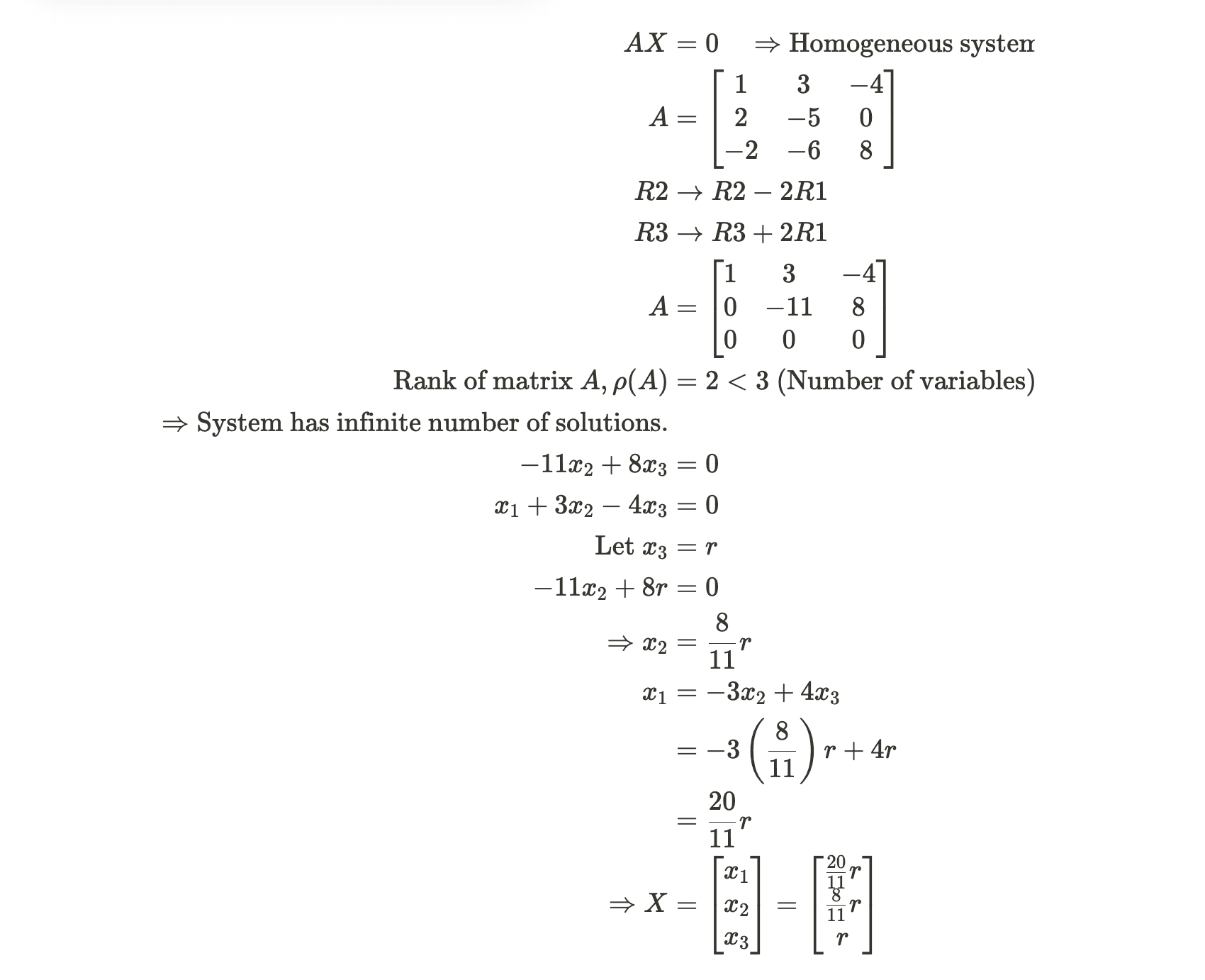
4. Find the solutions of above system of Linear equations

x1 + 3x2 − 4x3 = 0 2x1 − 5x2 = 0 −2x1 − 6x2 + 8x3 = 0

Answer

5. With no unique solution, solve for n with the following system of equations

Answer

n =5