3 Best Ways to Handle Right Skewed Data

Why is Normality so important?

Linear Discriminant Analysis (LDA), Linear Regression, and many other parametric machine learning models assume that data is normally distributed. If this assumption is not met, the model will not provide accurate predictions. 

What is normal distribution?

Normal distribution is a type of probability distribution that is defined by a symmetric bell-shaped curve. The curve is defined by its centre (mean), spread (standard deviation), and skewness.

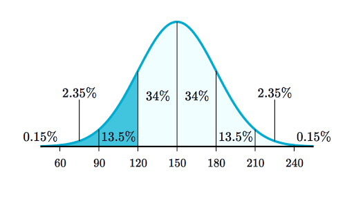
A normal distribution is the most common type of distribution found in nature. Many real-world phenomena, such as height, weight, and IQ, follow a normal distribution.

Normal distribution is important in statistics and is used to model many real-world phenomena. It is also used in quality control and engineering to determine acceptable tolerances.

What is skewness?

Skewness is the degree of asymmetry of a distribution. A distribution is symmetric if it is centred around its mean and the left and right sides are mirror images of each other. A distribution is skewed if it is not symmetric.

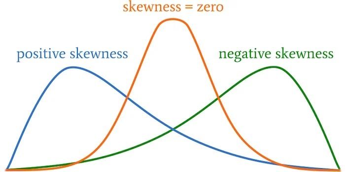
There are two types of skewness:

Positive Skewness: If the bulk of the values fall on the right side of the curve and the tail extends towards the right, it is known as positive skewness.

Negative Skewness: If the bulk of the values fall on the left side of the curve and the tail extends towards the left, it is known as negative skewness.

What does skewness tell us?

To understand this better consider a example:

Suppose car prices may range from 100k to 1,000,000 with the average being 500,000.

If the distribution’s peak is on the left side, our data is positively skewed and the majority of the cars are being sold for less than the average price.

If the distribution’s peak is on the right side, our data is negatively skewed and the majority of the cars are being sold for more than the average price.

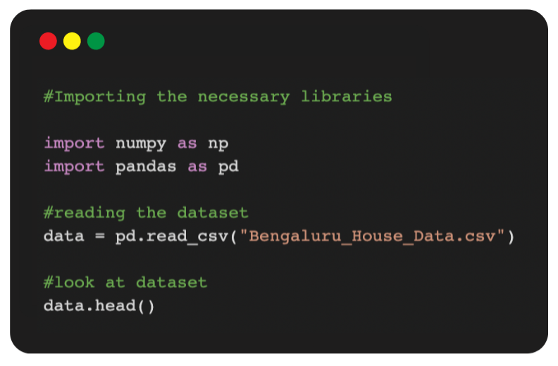
To experience what we have learned till now, we are going to work on a simple dataset.

The dataset used in this blog can be downloaded from the link given below: https://www.kaggle.com/datasets/amitabhajoy/bengaluru-house-price-data

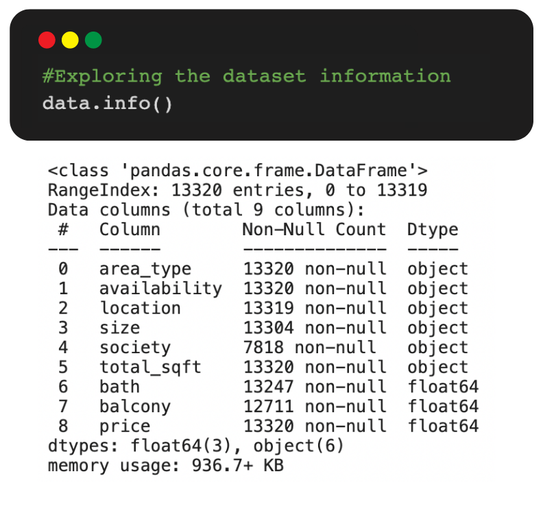
About Dataset:

We are going to use a dataset from Kaggle, which is a platform for Data Science communities. The dataset contains the prices of houses in Bengaluru, India.

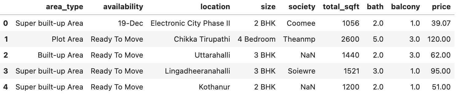
The dataset includes:

• Area Type: Type of plot
• Availability: Ready to move or not
• Location: Region of Bangalore
• Size: BHK
• Society: Colony in which the house is present
• Total Sq. Ft: Total area
• Bath: Number of bathrooms
• Balcony: Number of balconies
• Price: Cost in lakhs

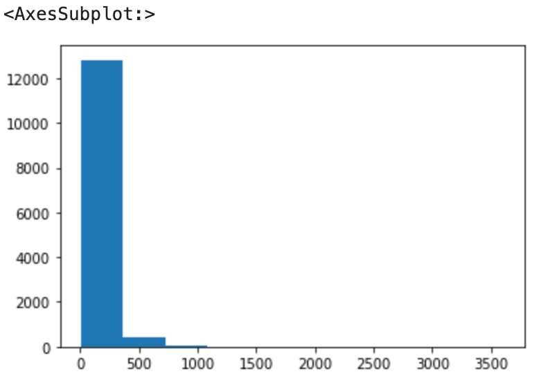
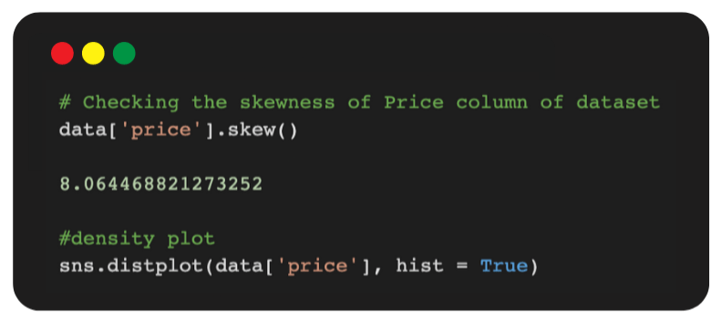
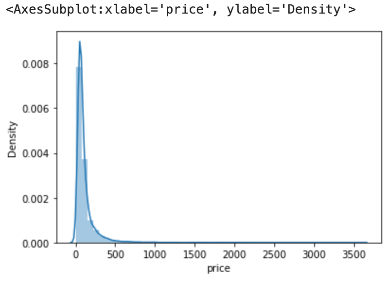
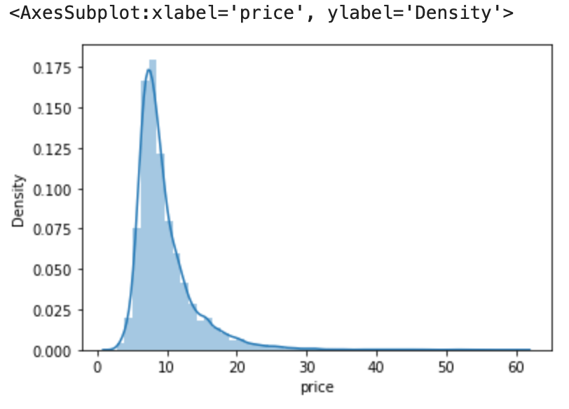
Note: As we can see the skewed values lie between -1 and greater than +1. Hence, data is heavily skewed. We can say that data[‘price’] is right skewed by looking at the graph and skewed values.

How to handle these skewed data?

- Transformation:

In data analysis, transformation is the replacement of a variable by a function of that variable. For example, replacing a variable x by the square root of x or the logarithm of x. In a stronger sense, a transformation is a replacement that changes the shape of a distribution or relationship.

• Steps to do transformation:

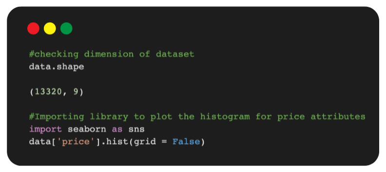
1. Draw a graph (histogram and density plot) of the data to see how far patterns in data match the simplest ideal patterns.
2. Check the range of the data. This is because transformations will have little effect if the range is small.
3. Check the skewness by statistical methods (decide right and left skewness).
4. Apply the methods (explained in detail below) to handle the skewness based on the skewed values.

To Handle Right Skewness

1. Log Transformation

The log transformation is widely used in research to deal with skewed data. It is the best method to handle the right-skewed data.

Why log?

The normal distribution is widely used in basic research studies to model continuous outcomes. Unfortunately, the symmetric bell-shaped distribution often does not adequately describe the observed data from research projects. Quite often, data arising in real studies are so skewed that standard statistical analyses of these data yield invalid results.

Many methods have been developed to test the normality assumption of observed data. When the distribution of the continuous data is non-normal, transformations of data are applied to make the data as “normal” as possible, thus, increasing the validity of the associated statistical analyses.

Popular use of the log transformation is to reduce the variability of data, especially in data sets that include outlying observations. Again, contrary to this popular belief, log transformation can often increase – not reduce – the variability of data, irrespective of whether or not there are outliers.

Why not?

Using transformations in general and log transformation in particular can be quite problematic. If such an approach is used, the researcher must be mindful about its limitations, particularly when interpreting the relevance of the analysis of transformed data for the hypothesis of interest about the original data.

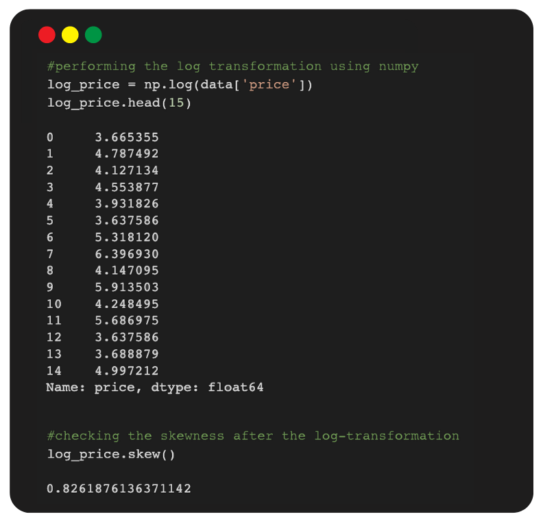
Note: Log transformation has reduced the skewed value from 8.06 to 0.82, which is nearer to zero.

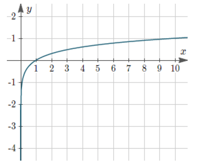
Note: If you’re getting the skewness value as nan, that means there are some values that are zero. In log transformation, it deals with only the positive and negative numbers, not with zero. The log ranges between (- infinity to infinity), however, it must be greater or less than zero. For better understanding, let’s have a look at the log graph below:

2. Root Transformation

2.1 Square root Transformation

• The square root means x to x^(1/2) = sqrt(x), is a transformation with a moderate effect on distribution shape. It is weaker than the logarithm and the cube root.
• It is also used for reducing right skewness, and has the advantage that it can be applied to zero values.
• Note that the square root of an area has the units of a length. It is commonly applied to counted data, especially if the values are mostly rather small.

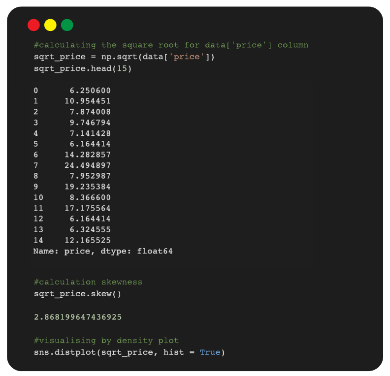
Note: In the previous case we got the skewness value as 0.82, but the square root transformation has reduced the skewed value from 8.06 to 2.86.

2.2 Cube root Transformation

The cube root means x to x^(1/3). This is a fairly strong transformation with a substantial effect on distribution shape.

• It is weaker than the logarithm but stronger than the square root transformation.
• It is also used for reducing right skewness, and has the advantage that it can be applied to zero and negative values.
• Note that the cube root of a volume has the units of a length. It is commonly applied to rainfall data.

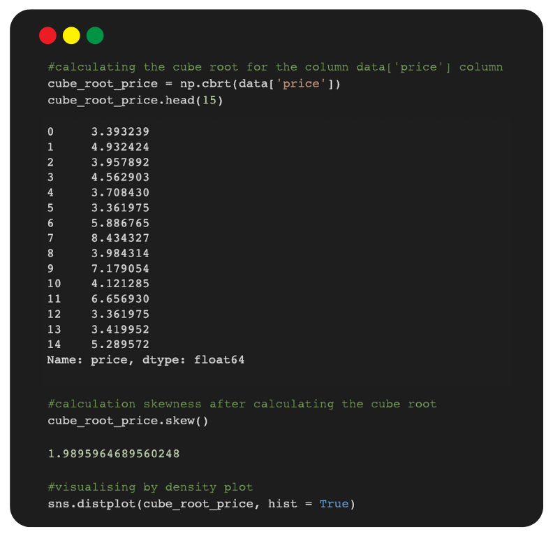
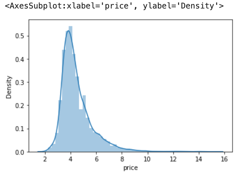
Note: In logarithm transformation, we got the skewness value as 0.82, and in the square root transformation it has reduced the skewed value from 8.06 to 2.86. However, now in the cube root transformation, the skewed values have reduced to 1.98 and it is near to zero compared to 2.86 and 8.06.

1. Reciprocals Transformation

The reciprocal, x to 1/x, with its sibling, the negative reciprocal, which is x to -1/x, is a very strong transformation with a drastic effect on distribution shape.

It cannot be applied to zero values. Although it can be applied to negative values, it is not useful unless all values are positive.

For example: we might want to multiply or divide the results of taking the reciprocal by some constant, such as 100 or 1000, to get numbers that are easy to manage, but that has no effect on skewness or linearity.

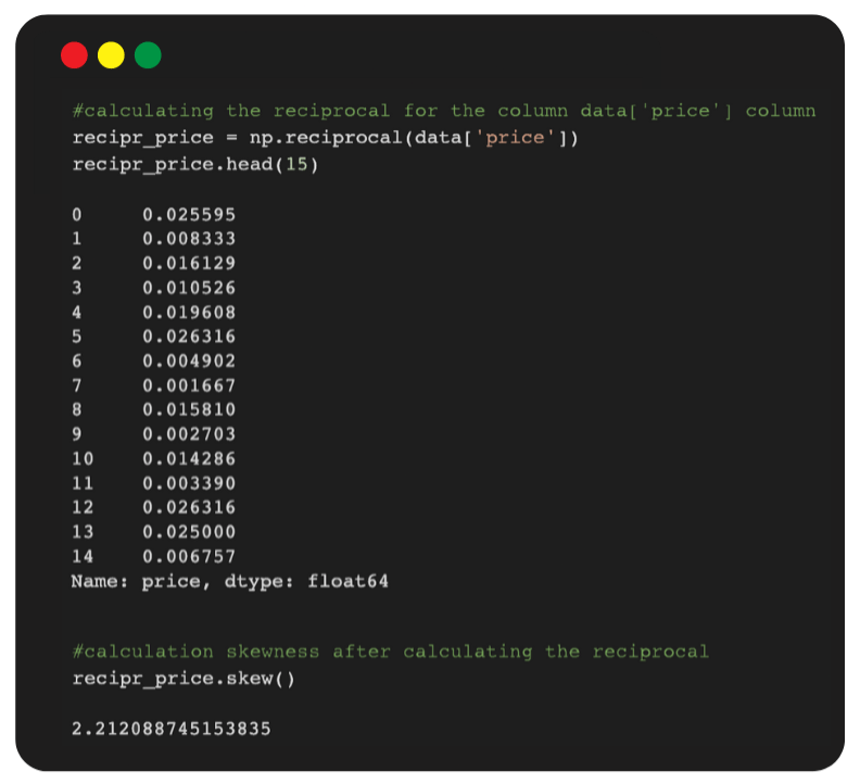
Note: In logarithm, square root, and cube root transformations, we got the skewness value as 0.82, 2.86 and 1.98 respectively. However, now in reciprocal transformation, the skewed value has reduced to 2.21 and it is near to zero compared to 2.86 and 8.06.

Therefore, we can conclude that log transformation has performed really well when compared to other methods by reducing the skewness value from 8.06 to 0.82.

Conclusion:

If you don’t deal with skewed data properly, it can undermine the predictive power of your model.

This should go without saying, but you should remember what transformation you have performed on which attribute, because you’ll have to reverse it when making predictions, so keep that in mind.

Nonetheless, these three approaches should be adequate for you.

If you are interested in pursuing a career in Data Science, enrol for our Full Stack Data Science program, where you will be trained from basics to advanced levels.

Read our recent blog on “Why do we always take p-value as 5%?”.