Excel for Data Analysis: The Top Formulas You Need to Know

If you’re a Data Analyst or aspiring to become one, it’s important to have a strong foundation in Excel and its various formulas.

In this blog, we will be covering the most essential formulas that you’ll need to know in order to effectively analyze data and make informed decisions. Whether you are just starting out with Excel or looking to refresh your skills, this blog is for you. We will be walking through each formula in detail, providing examples and tips on how to use them effectively. So let’s get started!

1. XLOOKUP:

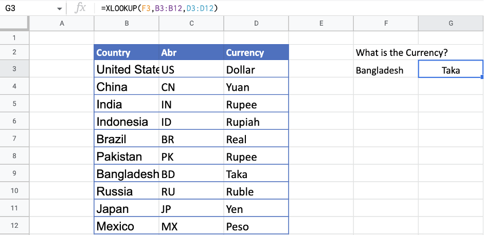
XLOOKUP is a newer function in Excel that can be used as an alternative to VLOOKUP or INDEX and MATCH. It allows you to search for a specific value in a table or range and return a corresponding value from the same row. The formula for XLOOKUP is as follows:

=XLOOKUP (lookup value, lookup array, return array)

In our example, as you can see we are using XLOOKUP to find the currency of Bangladesh by searching for the country name in cells B3:B12 and returning the corresponding currency from cells D3:D12.

1. IF, SUMIF, SUMIFS, COUNTIF, COUNTIFS, IFerror:

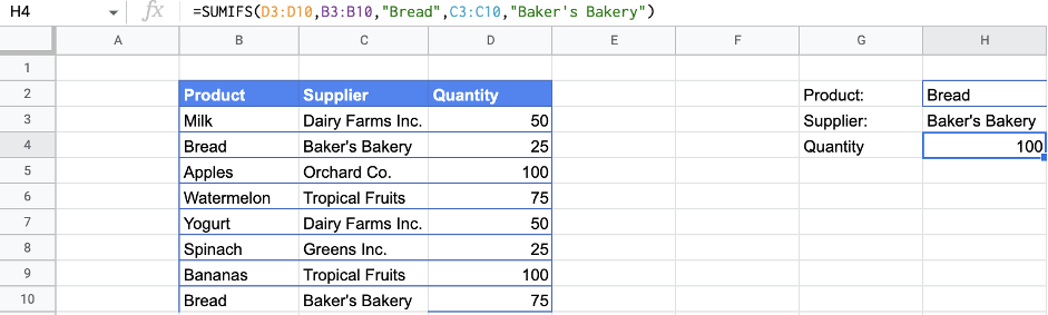
The basic functions of IF, SUMIF, SUMIFS, COUNTIF, and COUNTIFS. These functions are all used to perform calculations based on specified criteria.

IF is a logical function that returns one value if a condition is true and another value if the condition is false.

SUMIF and SUMIFS are used to sum values that meet specified criteria. SUMIF can only evaluate one criteria, while SUMIFS can evaluate multiple criteria from different columns. COUNTIF and COUNTIFS are similar to SUMIF and SUMIFS, but they count the number of cells that meet the specified criteria rather than summing their values.

IFERROR is a function that returns a specified value if a formula returns an error, and the original formula results if it does not. This can be useful for handling errors such as #DIV/0 or #VALUE! that may occur in a formula.

1. Transpose:

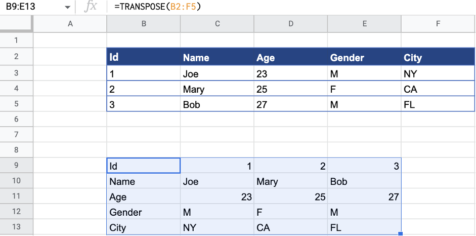
Transpose is a feature that allows you to rearrange the rows and columns of a data set. When you transpose a data set, the rows become columns and the columns become rows.

Select the data in the column: Click on the first cell in the column (for example, cell A1). Hold down the shift key and click on the last cell in the column (for example, cell A5). This will select all the cells in the column. Select the cell where you want the row to start: Click on the cell where you want the transposed data to appear (for example, cell B1). Right click and choose “Paste Special”: Right click on the cell you selected in step 2. From the menu that appears, choose “Paste Special.” Select transpose: In the “Paste Special” dialog box, check the box next to “Transpose.” Click “OK.”

This will transpose the data from the column to a row.

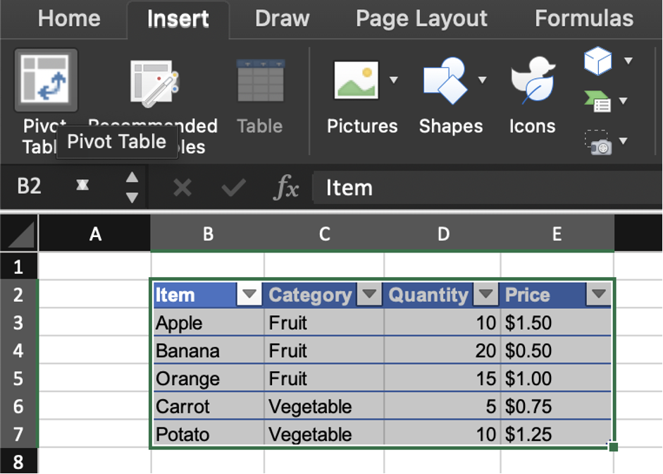
1. PIVOT TABLE:

Pivot tables are a powerful tool for analyzing and summarizing data. By selecting the fields we want to include in the pivot table and specifying how we want to organize and summarize the data, we can quickly and easily get a clear picture of our data to identify trends and patterns.

Pivot tables allow us to group data by a particular column, calculate sums or averages, find the maximum or minimum value, and more. We can also use pivot tables to create charts and graphs based on the summarized data, which can be helpful for visualizing and understanding our data.

Pivot tables are commonly used in business, finance, and other fields where large amounts of data need to be analyzed and summarized. They can be a valuable tool for anyone working with data, as they can help us quickly and easily get insights and understand trends and patterns in our data.

1. UPPER, LOWER, PROPER, TRIM:

The UPPER function in Excel converts a text string to all uppercase letters. For example, the formula =UPPER(“hello world”) would return “HELLO WORLD”.

The LOWER function converts a text string to all lowercase letters. For example, the formula =LOWER(“HELLO WORLD”) would return “hello world”.

The PROPER function converts a text string to proper case, which means the first letter of each word is capitalized and all other letters are lowercase. For example, the formula =PROPER(“hElLo WoRlD”) would return “Hello World”.

The TRIM function removes all spaces from a text string except for single spaces between words. For example, the formula =TRIM(" hello world ") would return “hello world”. These functions can be useful for cleaning up and standardizing text data in a spreadsheet.

Conclusion:

Excel is a powerful tool for data analysis that offers a wide range of formulas and features to help us organize, summarize, and analyze our data. In this blog, we covered some of the essential formulas we need to know in order to effectively analyze data and make informed decisions.

By mastering these formulas and features, we can effectively analyze and understand our data using Excel and make informed decisions. Whether we are just starting out with Excel or looking to refresh our skills, these formulas and features will be essential tools in our data analysis toolkit.

If you are an Excel enthusiast and want to explore a career in Data Science, sign up for our Full Stack Data Science program. New batch starts soon!

Read our recent blog on “How to become a Data Analyst without a degree and no experience”.