Linear Regression in Machine learning

Overview

Linear regression is an supervised learning technique in which it comes under regression technique. It is used when our dependent variable is continuous in nature. In this lesson we will learn about linear regression, it’s cost function, best fit line, etc.

Introduction to linear regression

Linear regression could be a statistical procedure utilized for predicting a reaction or dependent variable from one or more predictor or independent variables. It may be a sort of supervised learning algorithm that produces assumptions around the linear relationship between the input factors (x) and the single output variable (y). The objective of linear regression is to discover the best-fit line for the given information, so that ready to utilize it to anticipate the esteem of the output variable for any given input variable. Linear regression is the foremost commonly utilized predictive modelling procedure and can be utilized for both relapse and classification issues.

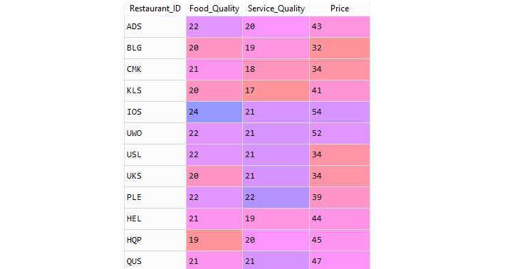
In the above dataset Price is the dependent variable(y) i.e. single output variable and Food_Quality and Service_Quality are independent variables that are input variables for our model and we can see the price data is continuous in nature.

What is Best Fit Line?

The best fit line is a line that summarizes the relationship between two variables in a linear regression model.

Types of Linear Regression

There are two types of linear regression:

1. Simple linear regression
2. Multiple linear regression

• Simple Linear Regression:

In simple linear regression, there is only one independent variable. The equation for a simple linear regression model is:

y = mx + b

where y is the dependent variable, x is the independent variable, m is the slope of the line, and b is the y-intercept. The slope (m) represents the change in y for every one-unit change in x, while the y-intercept (b) represents the value of y when x is equal to zero.

• Multiple Linear Regression:

In multiple linear regression, there are two or more independent variables. The equation for a multiple linear regression model is:

y = b0 + b1x1 + b2x2 + ... + bnxn

where y is the subordinate variable, x1, x2, ..., xn are the autonomous factors, and b0, b1, b2, ..., bn are the coefficients. The coefficients speak to the alter in y for each one-unit alter within the comparing autonomous variable, holding all other autonomous factors steady.

Hypothesis of Linear Regression

The hypothesis of linear regression is that there's a straight relationship between the autonomous variable(s) and the subordinate variable. In other words, it assumes that the alter within the subordinate variable is specifically relative to the alter within the independent variable(s).

Y = β0 + β1X1 + β2X2 + ... + βpXp + ε

where Y is the subordinate variable, X1, X2, ..., Xp are the autonomous factors, β0 is the intercept or constant term, β1, β2, ..., βp are the coefficients of the independent factors, and ε is the blunder term that speaks to the unexplained assortment inside the subordinate variable.

The speculation assumes that the mistakes are normally distributed, have a mean of zero, and have consistent variance (homoscedasticity). It also assumes that there's no multicollinearity (high correlation) between the independent variables.

Effect of Parameters

The parameters in linear regression are the coefficients (i.e., the weights) that are related with each include of the data set.The coefficients represent the relationship between the highlight and the dependent variable (i.e., the target).The affect of the parameters in linear regression is that they choose the quality and heading of the straight relationship between the highlights and the target. The more prominent the coefficient, the more grounded the relationship between the incorporate and the target. In case the coefficient is positive, it outlines that an increment inside the highlight is related with an increment inside the target; in case it is negative, it outlines that an increment inside the highlight is related with a reduce inside the target.

Error in Simple Linear Regression

Simple linear regression may be a statistical method utilized to foresee the values of one dependent variable based on the values of one autonomous variable. It may be a linear approach to modeling the relationship between two factors, where one variable is considered to be an explanatory variable (x) and the other is considered to be the response variable (y).

For illustration, a company may need to foresee the deals of a item based on the amount of cash went through on publicizing. In this case, the independent variable would be the publicizing budget and the dependent variable would be the deals of the item. The condition for basic linear regression is:

y = P0 + P1x

where P0 is the intercept (the value of y when x = 0), P1 is the slope of the line, and x is the value of the independent variable.

Choose parameters P1,P0 so that the predicted value h(x) is close to Y for our training examples (X,Y).

The sum of the squares of the residual errors are called the Residual Sum of Squares or RSS. The average variation of points around the fitted regression line is called the Residual Standard Error (RSE).

Cost Function in Simple Linear Regression

Choose parameters P1, P0 so that the predicted value h(x) is close to Y for our training examples (X,Y). The cost function helps us to figure out the best possible values for P0 and P1 which would provide the best fit line for the data points. Minimize the error between the predicted value and the actual value.

The Mean Squared Error (MSE) may be a degree of how close a predicted value is to the actual value. It is calculated by taking the contrast between the actual and predicted values, squaring the contrast, and after that taking the average of the squared differences. The smaller the MSE, the closer the anticipated values are to the genuine values.

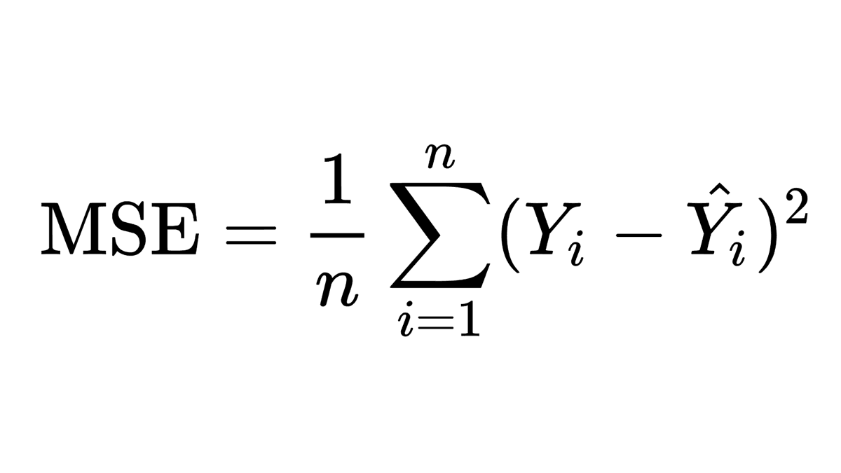
Where,

n = Number of observations 

ŷi = Predicted value for observation I 

yi = Actual value for observation i

Cost function

The cost function of multiple linear regression may be a degree of how exact the model is in foreseeing the target variable. It is calculated by taking the sum of the squared errors between the anticipated and real values.The cost function is expressed as:

J(θ) = 1/2m * Σi=1 to m (hθ(x(i)) - y(i))^2

where m is the number of training examples, θ is the vector of model parameters, hθ(x(i)) is the hypothesis function evaluated at x(i), and y(i) is the target value for x(i).

Assumptions of linear regression

It is additionally vital to check for presumptions of linear regression. On the off chance that these assumptions are not met, at that point linear regression might not be suitable, and other regression models or machine learning algorithms ought to be considered.

1. Linearity: The relationship between the independent and dependent variables should be linear. This will be checked by plotting a scatterplot of the two factors and visually assessing the pattern of the data points.
2. No multicollinearity: The independent variables ought to not be exceedingly correlated with each other. This could be checked by computing the correlation matrix of the independent variables, and looking for values greater than 0.7 or less than -0.7.
3. Homoscedasticity: The variance of the residuals ought to be constant across all values of the independent variables. This may be checked by plotting the residuals against each of the independent variables and trying to find a design within the spread of the points.
4. No autocorrelation: The residuals ought to be independent from one another. This could be checked by computing the autocorrelation function of the residuals and seeking out for significant values.
5. Normality: The residuals should be normally distributed. This can be checked by plotting a histogram of the residuals and visually inspecting the shape of the distribution.

Linearity

Before using linear regression algorithm, it is important to check if there is a linear relationship between the independent variable(s) and the dependent variable. One way to check for linearity is to use scatter plots to visually inspect the relationship between the variables.

1. If the scatter plot shows a roughly linear pattern, then linear regression might be appropriate. If there is no clear pattern or if the pattern is nonlinear, then linear regression might not be the best approach.
2. Another way to check for linearity is to compute the correlation coefficient between the independent variable(s) and the dependent variable. The correlation coefficient measures the strength and direction of the linear relationship between two variables. If the correlation coefficient is close to 1 or -1, then there is a strong linear relationship. If the correlation coefficient is close to 0, then there is little or no linear relationship.

Multicollinearity

Multicollinearity is a phenomenon in which two or more predictor variables in a multiple linear regression model are highly correlated. This means that one or more of the predictor variables can be linearly predicted from the others with a substantial degree of accuracy.

Multicollinearity is a problem because it reduces the accuracy of the regression coefficients and makes it difficult to interpret the results. For example, if two predictor variables are highly correlated, then one of them may be redundant and can be removed from the model without significantly affecting the model's accuracy.

1. To detect multicollinearity, one can calculate the variance inflation factor (VIF), which measures the degree of correlation between each predictor variable and all the other predictor variables. A VIF score of greater than 5 indicates that multicollinearity is present.

VIF= 1/1-Ri^2

2. Multicollinearity can be addressed by using a technique called regularization, which involves adding a penalty term to the regression model that penalizes large values of the regression coefficients. This helps to reduce the influence of highly correlated predictor variables on the model. In addition, one can also use feature selection techniques to select a subset of uncorrelated predictor variables.

What is Homoscedasticity and Heteroscedaticity?

Homoscedasticity and heteroscedasticity are terms used to describe the variance of errors in a regression model.

1. Homoscedasticity, moreover known as constant variance, happens when the change of blunders is the same for all values of the independent variable(s). In other words, the spread of residuals is reliable over the range of anticipated values. Usually desirable because it shows that the changeability within the subordinate variable isn't changing as a function of the autonomous variable(s), and the show is more solid for making predictions. 
2. Heteroscedasticity, on the other hand, happens when the variance of mistakes isn't consistent over the range of the independent variable(s). This implies that the spread of residuals isn't reliable, and the variability of the subordinate variable changes as a work of the autonomous variable(s). Heteroscedasticity can lead to one-sided and inefficient estimates of the regression coefficients, and it can influence the unwavering quality of the model for making expectations. 
3. Heteroscedasticity can regularly be recognized by visual review of a plot of the residuals against the anticipated values. In the event that the spread of the residuals is reliable over the range of predicted values, at that point the information is likely homoscedastic. On the off chance that the spread of residuals is more extensive or smaller for certain anticipated values, at that point the information is likely heteroscedastic.

There are a few strategies for managing with heteroscedasticity, including transforming the data, utilizing weighted least squares, or employing a different regression model altogether, such as a robust regression model.

Residual analysis

Residual analysis is an important step in linear regression. It helps to identify potential problems with the linear regression model, such as outliers, non-linearity, and heteroscedasticity.

An equation for residual analysis is as follows:

Residual = Observed Value - Predicted Value

An example of residual analysis would be fitting a linear regression model to predict the price of a house based on its square footage. After the model is fit, we can calculate the residuals for each house by subtracting the predicted price from the observed price. If we find that the residuals are not randomly distributed around zero, then this could indicate that the linear regression model is not the best fit for this dataset.

Normality

Normality is an assumption of linear regression that states that the errors or residuals of the model are normally distributed. In other words, the distribution of the residuals should follow a normal or Gaussian distribution with a mean of zero.

Normality is important because it affects the reliability and accuracy of the estimated regression coefficients and predictions. When the residuals are normally distributed, it means that the model is correctly accounting for all the factors that affect the dependent variable, and that there are no systematic errors in the model.

Normality can be assessed by examining a histogram or a Q-Q plot of the residuals. A histogram of the residuals should show a roughly symmetrical distribution around zero, and a Q-Q plot should show the residuals following a straight line. If the histogram or Q-Q plot shows significant deviation from normality, then the model assumptions may not be met.

If the normality assumption is not met, several transformations can be applied to the data to make the residuals more normally distributed. Common transformations include logarithmic, exponential, and Box-Cox transformations. Alternatively, a non-linear regression model or a robust regression model that does not rely on normality assumptions can be used.

Outlier detection

Outlier detection in linear regression is a process of identifying and removing or adjusting outliers in a data set that may produce misleading results during linear regression analysis. Outliers are observations that are significantly different from the remaining observations in a dataset. Outliers may be the result of data entry errors, measurement errors, or extreme values that do not reflect the true underlying pattern of the data.

Outliers can have a large influence on the results of linear regression. For example, if we have a data set with 10 observations, and one of the observations is an outlier, it can affect the slope and intercept of the regression line. To detect and remove outliers, we can use the following methods:

1. Visualization: We can plot the data and look for points that are far away from the regression line.
2. Residual Analysis: We can use a scatter plot of the residuals to identify outliers. Residuals are the differences between the observed values and the predicted values. Outliers are usually identified as observations that have a large residual value.
3. Standardized Residuals: We can calculate a standardized residual for each observation and identify any observation with a standardized residual greater than two or three as an outlier.

Once outliers have been identified, they can be removed or adjusted. For example, if the outlier is due to data entry errors, it can be corrected. If the outlier is due to extreme values, it can be adjusted to a more reasonable value.

Model selection

When selecting a model for linear regression, it is critical to consider the sort of information that's being utilized, the number of factors, and the reason of the examination.

1. Type of Data: The sort of information being utilized ought to be taken into thought when selecting a model. In the event that the information is continuous, at that point a linear regression model may be the finest choice. In the event that the data is categorical, at that point a logistic regression model maybe a better choice.
2. Number of Variables: The number of variables ought to too be taken into consideration when selecting a model. In the event that there are a expansive number of factors, at that point a regularized regression may be the finest choice. Regularized regression procedures, such as ridge regression, can offer assistance decrease the hazard of overfitting due to high collinearity.
3. Purpose: The purpose of the examination ought to moreover be considered when selecting a model. In the event that the objective is to form predictions, at that point a linear regression model may be the most excellent choice. In any case, on the off chance that the objective is to understand the relationships between the factors, at that point a more complex model such as a stepwise regression may be a way better choice.

Eventually, the sort of data, the number of variables, and the reason of the analysis ought to all be taken into thought when selecting a show for linear regression.

Applications of linear regression

Common applications of linear regression incorporate predicting future stock costs, estimating deals, anticipating client churn, understanding the affect of showcasing campaigns, and predicting housing costs. Linear regression can too be utilized to decide the connections between distinctive features in a dataset, and it is commonly utilized in predictive analytics and data mining. It can moreover be utilized to decide the affect of changes in inputs on a model's output, and to distinguish correlations between different variables.

Conclusion

The industry utilized linear regression to foresee the cost of a house given the highlights of the domestic. By preparing a model on a set of known domestic costs, the model was able to accurately predict the cost of a unused home based on its features. This model has been effectively connected within the housing market and has been utilized to assist buyers and venders make educated choices approximately the esteem of a particular home.

Key takeaways

1. Linear regression could be a supervised machine learning algorithm utilized to foresee a continuous numerical value.
2. Linear regression employs a linear equation to approximate the relationship between independent variables and the dependent variable.
3. Linear regression may be a effective tool for anticipating quantitative results.
4. Linear regression requires a linear relationship between the independent variables and dependent variable.
5. The model produced by linear regression can be utilized to form predictions around the dependent variable.
6. Linear regression can be utilized to distinguish vital features that impact the dependent variable.
7. Assumptions such as linearity of the data, normality of the errors, and homoscedasticity are fundamental for precise linear regression models.
8. Regularization strategies such as L1 and L2 can be utilized to diminish overfitting and improve predictive accuracy.

Quiz

1. What does the coefficient of determination (R-squared) measure? 
   1. The amount of variability in the data 
   2. The strength of the linear relationship between two or more variables 
   3. The number of observations in a dataset  
   4. The slope of the regression line

Answer: b. The strength of the linear relationship between two or more variables

2. When is linear regression used?  
   1. To predict a categorical variable  
   2. To explain the relationships between two or more variables 
   3. To predict a continuous variable 
   4. To identify outliers

Answer: c. To predict a continuous variable

3. Which of the following is a disadvantage of linear regression?  
   1. It is not suitable for predicting non-linear relationships  
   2. It does not require any assumptions about the data 
   3. It does not require a large dataset 
   4. It is not suitable for making predictions

Answer: a. It is not suitable for predicting non-linear relationships

4. What is the goal of linear regression? 
   1. To identify outliers 
   2. To explain the relationships between two or more variables  
   3. To predict a continuous variable 
   4. To minimize the cost of the model

Answer: c. To predict a continuous variable