How to Detect Outliers in Machine Learning? (With Examples)

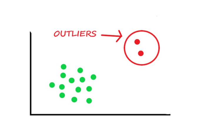
An outlier in data analysis might be a rotten apple in a dataset of quality apples. While the vast majority of apples in the dataset may have a high-quality rating, the presence of a single rotten apple can significantly impact the overall average quality rating for the entire dataset. Outlier detection techniques can be used to identify and remove this "rotten apple" outlier, allowing for more accurate and reliable data analysis.

Now coming to handling this “rotten apple” efficiently and rightly, the most obvious solution you may think of is to remove the rotten apple. Similarly, in data analysis, we have different types of handling the outliers in the data to enhance data analysis. Along with statistical methods, some Machine Learning techniques include supervised, semi-supervised, and unsupervised methods to handle outliers.

This article includes the following:

• What is outliers in machine learning and why do we need to detect outliers?
• Different outlier detection methods in machine learning
• Outlier detection using standard deviation
• Z score outlier detection
• Interquartile range outlier detection
• Outlier Detection using percentile

What are Outliers in Machine Learning and Why do We need to Detect Outliers?

Let’s understand what are outliers in machine learning and what is outlier detection in machine learning. An outlier is a data point significantly different from other data points in a dataset. Outliers can occur for various reasons, such as measurement errors, data entry errors, or natural variations in the data. They can significantly impact the outlier analysis in machine learning and interpretation of the data, so it is essential to detect them.

Outliers can be detected using various methods, such as visual inspection of the data, statistical measures such as the Z-score or the interquartile range, or machine learning techniques. Once outliers are detected, they can be handled in various ways, such as removing them from the dataset, replacing them with the mean or median of the data, using outlier detection techniques using machine learning, or using algorithms that are less sensitive to outliers.

Outlier Detection

Detecting outliers is crucial because they can distort the overall picture of the data and lead to incorrect conclusions if not appropriately handled. Outliers can also affect the performance of many machine learning models, as they can skew the results and lead to overfitting or poor generalization. Thus, detecting outliers is essential for cleaning and preparing the data for analysis and ensuring the results’ validity.

Different Outlier Detection Methods in Machine Learning

There are various outlier detection techniques in machine learning that are categorized as supervised methods, semi-supervised methods, and unsupervised methods. The below image shows a list of a few ways on how to detect outliers in machine learning under the three categories.

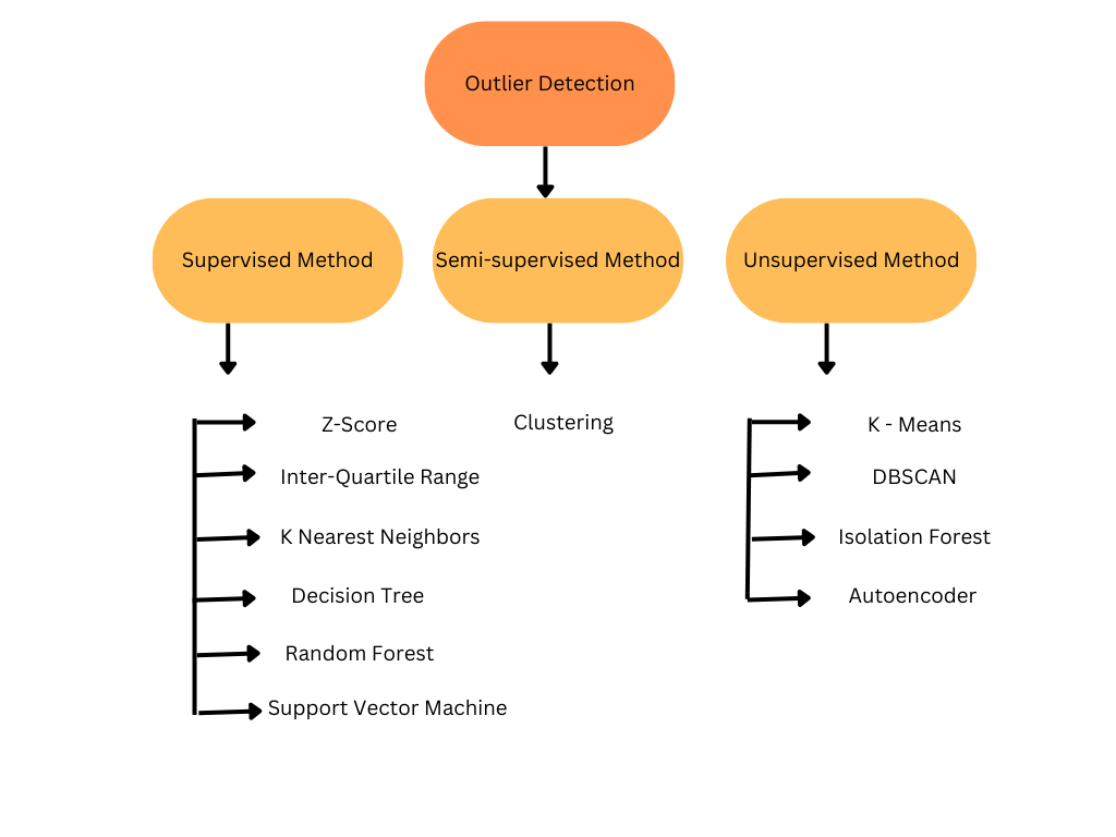
Outlier Detection in Machine Learning

1. Supervised methods: These methods use labeled data to identify outliers. For example, a supervised outlier detection algorithm may use a decision tree or a random forest to classify data points as outliers or non-outliers based on the features of the data.

2. Semi-supervised methods: These methods use a combination of labeled and unlabeled data to identify outliers. For example, a semi-supervised outlier detection algorithm may use clustering to group similar data points together and then use the labeled data to identify outliers within the clusters.

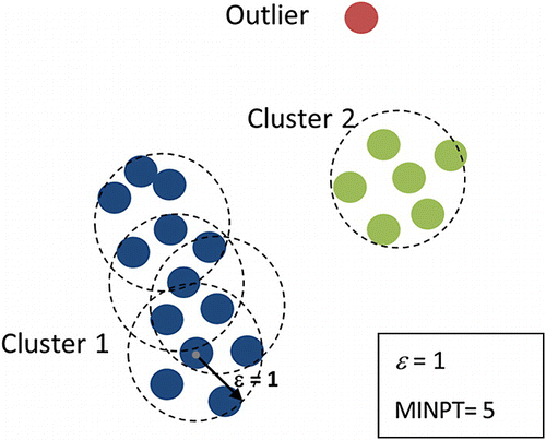
Outliers within the Clusters

3. Unsupervised methods: These methods use only unlabeled data to identify outliers. For example, unsupervised outlier detection methods can use density-based or distance-based methods to identify data points that are far away from the rest of the data. Some popular unsupervised methods include the Local Outlier Factor (LOF), k-nearest neighbor (KNN) based method, DBSCAN, and Isolation Forest.

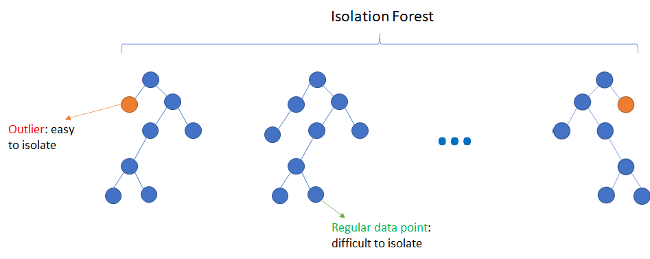
Isolation Forest

In addition to these three main categories, there are also other methods for outlier detection, such as ensemble methods that combine multiple methods or deep learning-based methods that use neural networks to identify outliers.

It is necessary to note that the method for outlier detection will depend on the specific characteristics of the data and the problem at hand. It’s also important to consider the trade-off between computational cost and the accuracy of outlier detection.

We will see some of the primary methods for outlier detection with practical implementation.

Outlier Detection using Standard Deviation:

A straightforward method for detecting outliers using standard deviation is to calculate the standard deviation of the data and then identify data points that fall outside of a certain number of standard deviations from the mean.

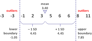
Standard Deviation

Example of using Standard Deviation

For example, let us do a practical implementation by generating a random dataset using the NumPy library and performing outlier detection.

Step1: Importing the required Libraries

# Importing Required Libraries 
import pandas as pd
import numpy as np

import matplotlib.pyplot as plt
import seaborn as sns

Step2: Collecting the data

mean=30,
std dev = 5
samples 100
#generating a random normally distributed data 
age_data = np.random.normal(loc=mean, scale=std_dev, size=samples)

#rounding up the values to 8 decimal places 
age_data = np.round(age_data, decimals=0) 
age_data = age_data.tolist() # converting the array to list
print (age_data)

This will generate a dataset of 100 ages that have a mean of 30 and a standard deviation of 5, which approximates a normal distribution. As you can observe above, the ages generated are random numbers and not people’s actual ages.

It’s important to note that real-world datasets usually don’t follow a perfect normal distribution but may be close to normal distribution. In such cases, it’s essential to check the distribution of the data using tools such as histograms and probability plots to check how well the data follows a normal distribution.

It’s important to note that this method assumes that the data is normally distributed. If the data is not normally distributed, this method may not be appropriate, and other methods should be considered.

Step3: Visualize the data

# Visualise the data
sns.set_theme() 
sns.displot(data-age_data).set(title="Distribution of Age",xlabel="Age") 
plt.show()

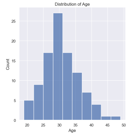
Distribution of Age

From the above plot, it is clearly visible that our data is normally distributed. Hence, we can use the standard deviation method to detect the outliers. We must note that if our data is not normally distributed, we need to use other methods for detecting outliers.

Now, we will use this data throughout this tutorial.

#Calculate the mean and standard deviation
mean = np.mean(age_data) 
std_dev = np.std(age_data)

# Set a threshold for the number of standard deviations away from the mean threshold = 2

#Identify outliers 
outliers1 = []
for age in age data: 
    if abs(age - mean)> threshold * std_dev:
       outliers.append(age)
       
print("Outliers:7, outliers1)

In the below example of data containing heights, we can see how the number of outliers vary depending on the threshold value we choose.

Example

Hence, depending on the use case, it is crucial to choose the right threshold.

Z score Outlier Detection

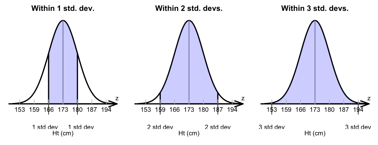
The Z-score method for outlier detection uses a dataset’s standard deviation and its mean to identify data points that are significantly different from the majority of the other data points.

Let’s now examine the Z-score notion. The Z-score for a value of x in the dataset with a normal distribution with mean μ and standard deviation σ is given by:

z = (x - μ)/σ

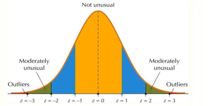
Z-score takes the following values as shown below:

The Z-score is equal to zero when x = .μ The Z-score is ± 1, ± 2, or ± 3, depending on whether x is ± 1, ± 2, or ± 3, respectively.

Example

A data point with a Z-score (the number of standard deviations the data point is away from the mean) of more than 3 or less than -3 is typically considered to be an outlier. This method assumes that the data follows a normal distribution. It is a simple and widely used method for outlier detection, but it may not always be appropriate for data that is not normally distributed.

Example of using Z-score:

We will use the same age_data we previously used to implement Z score outlier detection.

First, we need to get the mean and standard deviation of the dataset.

mean
 = np.mean (age_data)
std = np.std(age_data)
print('mean of the dataset is', mean) 
print('std. deviation is', std)

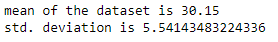
We can observe that the mean and standard deviation are 30.15 and 5.5, respectively.

Now, we need to calculate the Z-score for each of the data points. And then, the data points that have Z-score more than +3 or less than -3 are considered outliers.

threshold = 3
outlier2 = [] 
for i in age_data:
    z= (i-mean)/std 
    if z > threshold:
       outlier.append(i)
print('outlier in dataset is', outlier2)

Using this method, we can observe that we have got only one value, i.e., 49, as an outlier.

Interquartile Range Outlier Detection

(IQR) Interquartile Range outlier detection method involves calculating the first and third quartiles (Q1 and Q3) of a dataset and then identifying any data points that fall beyond the range of Q1 - 1.5 * IQR to Q3 + 1.5 * IQR, where IQR is the difference between Q3 and Q1. Data points that fall outside of this range are considered outliers.

The below image gives a clear view of the detection of outliers using the Interquartile Range.

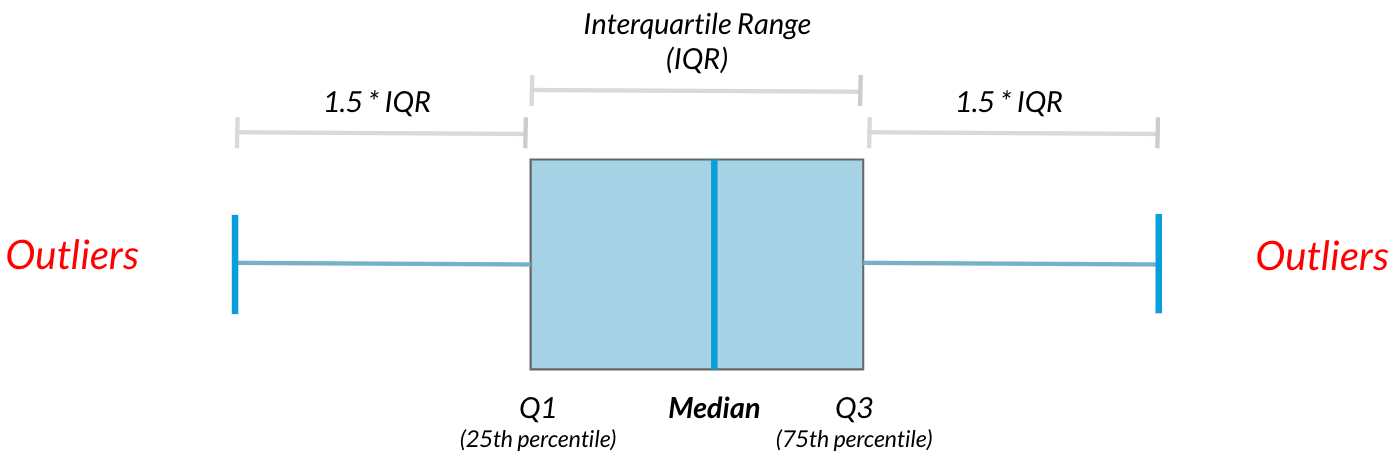
Interquartile Range

Example of using Interquartile Range (IQR):

To use the IQR method, let us first sort the data in ascending order.

# Take the data and sort it in ascending order. 
sort_data = np.sort(age_data)
sort data 

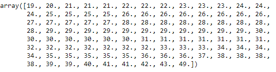
The above snippet of code ensures that our data is sorted.

We can visualize using the boxplot graph to get a better picture of the data.

sns.boxplot(data-sort_data).set(title="Box Plot of Age")
plt.show()

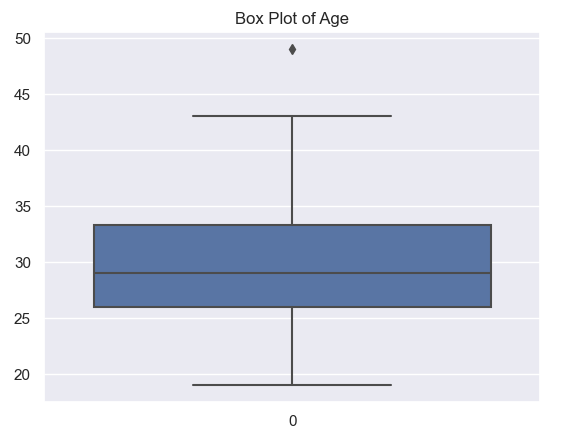
Box Plot of Age

The boxplot shows that there is one outlier in the data.

Now, we will calculate the different quartiles to find the IQR.

Calculate Q1, Q2, Q3 and IQR.

Q1 = np.percentile(sort_data, 25, interpolation = 'midpoint')
02 = np.percentile(sort_data, 50, interpolation = 'midpoint') 
Q3 = np.percentile(sort_data, 75, interpolation = 'midpoint')

print('Q1 25 percentile of the given data is, ', Q1)
print('Q1 50 percentile of the given data is, ', Q2)
print('Q1 75 percentile of the given data is, ', Q3)

IQR = Q3 - Q1 
print('Interquartile range is', IQR)

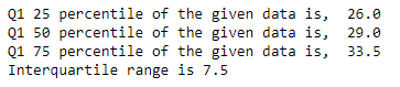
We can also directly calculate the IQR using the following code:

q25,q75 = np.percentile (a = age_data, q=[25,75])
iqr = q75 - 925

Now that we know our IQR, let’s calculate the upper and lower limit to find our outliers that lie below and above the boundaries we obtained.

low_lim =  Q1 - 1.5 * IQR 
up_lim = Q3 - 1.5 IQR

print('low_limit is', low_lim) 
print('up_limit is', up_lim)

low_limit is 14.75

up_limit is 44.75

We can now find the data points that fall outside the limits we obtained.

outlier3 [] 
for x in sort_data:
    if ((x> up lim) or (x<low_lim)):
        outlier3.append(x) 
print(" outlier in the dataset is", outlier3)

outlier in the dataset is [49.0]

There is one data point in the data, which is an outlier that falls outside the limits.

Outlier Detection using Percentile

Outlier detection using percentiles involves identifying data points that fall outside a specific range of percentiles. The range of percentiles can be specified as a percentage of the data, such as the top and bottom 5% of data points. Data points that fall outside of this range are considered outliers.

Example of using Percentile

The percentile method is similar to the IQR method.

Here, we will consider the top and bottom 5% of data points as outliers and find the upper and lower limit.

lower lim = np.percentile(a = age_data, q= 5)
upper lim = np.percentile(a = age data, q = 95) 
print('lower limit is', lower lim) 
print('upper limit is', upper lim

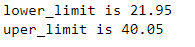
Using the limits we obtained, we can get the data points that fall outside the boundaries.

outlier4 =[]
for x in age_data: 
    if ((x) upper lim) or (x<lower_lim)):
         outlier4.append(x)
print('outliers in the dataset are', outlier4)

Note that the percentile we choose will depend on the data and the domain we are working on.

Outlier detection helps to identify data points that are unusual or do not conform to the expected pattern in a dataset. Several other methods are available for outlier detection, including statistical methods and machine learning techniques. Statistical methods such as Z-score and the modified Z-score method commonly identify outliers. Machine learning methods such as Local Outlier Factor (LOF) and one-class SVM are some methods for outlier detection. These methods are effective in identifying outliers in high-dimensional datasets. However, it is essential to note that not all outliers are errors, and care should be taken in interpreting the results of outlier detection.

If Data Science is a field that intrigues your professional interests, then sign up for our Full Stack Data Science course that offers 100% placement guarantee at top product and service companies.