Supervised Learning for GATE Exam

Supervised learning is a fundamental concept in machine learning where the algorithm learns to make predictions or decisions based on input data by being provided with a labeled dataset during training. In supervised learning, the "supervisor" provides the algorithm with a clear mapping between input and output, which allows the algorithm to learn patterns and relationships in the data. The main components of supervised learning are:

• Input Data (Features): These are the variables or attributes that the algorithm uses to make predictions. They are also called the independent variables or input features.
• Output Data (Labels or Targets): These are the desired outcomes or predictions that the algorithm is expected to generate based on the input data. Labels are also known as dependent variables or output targets.
• Training Data: This is the labeled dataset used to train the model. It consists of input-output pairs, where the algorithm learns to associate inputs with their corresponding outputs.
• Algorithm (Model): The algorithm or model used in supervised learning learns to map input data to output data. The goal is to find a function that approximates this mapping, making accurate predictions for new, unseen data.
• Loss Function: A loss function quantifies the error between the model's predictions and the actual labels in the training data. The model aims to minimize this error during training.
• Optimization: Optimization techniques like gradient descent are used to update the model's parameters iteratively, improving its predictive performance.

Importance of Supervised Learning

Supervised learning is crucial in machine learning for several reasons:

• Predictive Power: It enables machines to make predictions or classifications, which has wide-ranging applications in various fields, including healthcare, finance, and natural language processing.
• Automation: It allows for the automation of decision-making processes based on historical data, reducing human intervention and error.
• Personalization: Supervised learning is essential for building recommendation systems that personalize content and product recommendations for users.
• Pattern Recognition: It helps identify and understand patterns and relationships in data, which can be valuable for data analysis and business insights.

1. Differentiation between Supervised, Unsupervised, and Reinforcement Learning:
   • Supervised Learning: As explained above, supervised learning involves training a model on labeled data, with a clear mapping between input and output. It's used for tasks like classification and regression.
   • Unsupervised Learning: Unsupervised learning deals with unlabeled data, where the algorithm explores the data's inherent structure or patterns without explicit guidance. Common techniques include clustering (grouping similar data points) and dimensionality reduction (reducing the complexity of data while preserving important features).
   • Reinforcement Learning: Reinforcement learning is a type of machine learning where an agent interacts with an environment and learns to make a sequence of decisions to maximize a cumulative reward. It involves trial-and-error learning and is commonly used in robotics, game playing, and autonomous systems.
2. Examples of Supervised Learning Applications:
   • Email Spam Detection: Supervised learning models can be trained to classify emails as either spam or not spam based on the content and attributes of the emails.
   • Handwriting Recognition: Supervised learning can be used to build character recognition systems that convert handwritten text into digital text.
   • Credit Scoring: Banks and financial institutions use supervised learning to assess the creditworthiness of applicants by predicting their likelihood of defaulting on loans based on historical data.
   • Medical Diagnosis: Supervised learning models can assist doctors in diagnosing diseases by analyzing patient data, such as medical images or lab results, to predict specific medical conditions.
   • Language Translation: Machine translation systems like Google Translate use supervised learning to translate text from one language to another by learning from parallel text corpora.
   • Autonomous Vehicles: Self-driving cars employ supervised learning for tasks such as object detection and lane following, using labeled data to make real-time driving decisions.

These examples illustrate the versatility and significance of supervised learning in a wide range of applications across various domains.

Types of Supervised Learning

Regression and Classification are two main types of supervised learning in machine learning, and they serve different purposes based on the nature of the output variable they aim to predict:

Regression:

• Purpose: Regression is used when the output variable is continuous or numeric, meaning it can take any value within a certain range. The goal of regression is to model the relationship between input variables and the continuous output, enabling predictions of real-valued quantities.
• Output: The output of a regression model is a continuous value or a numerical prediction. It represents a quantity on a scale.
• Examples:
  • Predicting house prices based on features like square footage, number of bedrooms, and location.
  • Estimating the temperature based on historical weather data and time of day.
  • Predicting a person's age based on demographic features such as height, weight, and income.

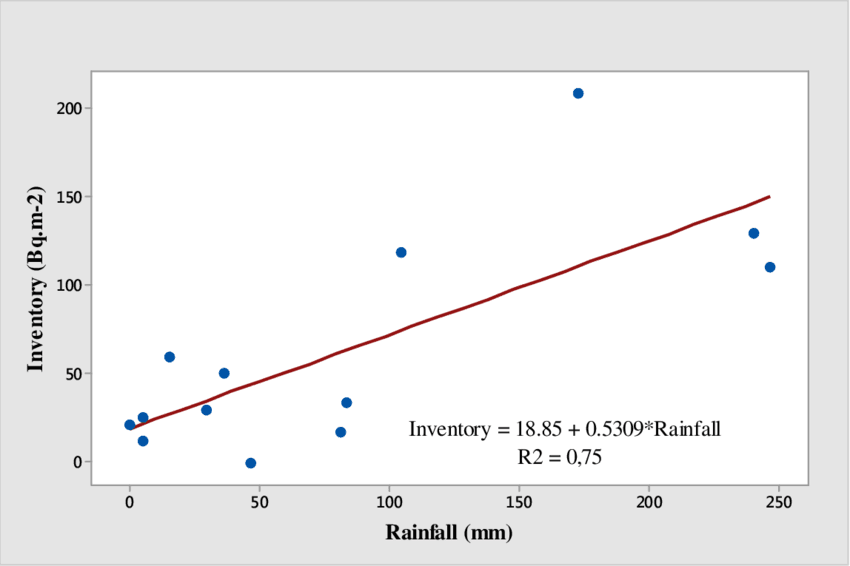
Regression Example

Classification:

• Purpose: Classification is used when the output variable is categorical, meaning it falls into predefined classes or categories. The goal of classification is to learn a mapping from input features to discrete class labels, allowing the model to assign new data points to one of these categories.
• Output: The output of a classification model is a discrete class label or category. It represents a class membership or category assignment.
• Examples:
  • Spam Email Detection: Classifying emails as "spam" or "not spam."
  • Image Classification: Identifying whether an image contains a cat, dog, or some other object.
  • Disease Diagnosis: Categorizing patients as "healthy," "mildly ill," or "severely ill" based on medical test results.
  • Sentiment Analysis: Determining the sentiment of a text as "positive," "negative," or "neutral."

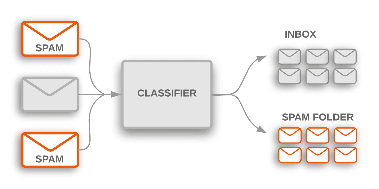
Classification Example

Key Differences:

• Nature of Output: The main difference between regression and classification is the nature of the output variable. In regression, the output is continuous and can take any value within a range, while in classification, the output is categorical and belongs to a predefined set of classes.
• Use Case: Regression is suitable for problems where you want to predict a quantity, such as a price, temperature, or age, based on input features. Classification, on the other hand, is used when you want to categorize data into distinct groups or classes.

Examples:

1. Regression Problem:
   • Problem: Predicting a house's sale price based on various features.
   • Input Features: Square footage, number of bedrooms, number of bathrooms, neighborhood, etc.
   • Output: The predicted sale price, which is a continuous numerical value.
2. Classification Problem:
   • Problem: Identifying whether an email is spam or not.
   • Input Features: Email content, sender information, subject line, etc.
   • Output: A binary classification where the output is either "spam" or "not spam."
3. Regression Problem:
   • Problem: Predicting a person's annual income based on demographic data.
   • Input Features: Age, education level, occupation, marital status, etc.
   • Output: The predicted annual income, which is a continuous numerical value.
4. Classification Problem:
   • Problem: Identifying handwritten digits (0-9) in an image.
   • Input Features: Pixel values of the image.
   • Output: A multi-class classification where the output is one of the digits (0, 1, 2, ..., 9).

These examples illustrate the fundamental differences between regression and classification, showcasing their respective applications and the types of output they generate.

Linear Regression

Linear Regression is one of the most fundamental and widely used regression algorithms in machine learning. It's used for modeling the relationship between a dependent variable (also known as the target or output) and one or more independent variables (features or predictors) by fitting a linear equation to the observed data. Linear regression is primarily used for predicting a continuous output.

Here are the key components of a linear regression model:

1. Linear Regression Model:

• In simple linear regression, there is one independent variable (feature) and one dependent variable (output).
• The model assumes a linear relationship between the independent variable(s) and the dependent variable. Mathematically, it can be represented as:
  y=b0+b1x
• y represents the dependent variable (output).
• x represents the independent variable (feature).
• b0 is the intercept (the value of y when x is 0).
• b1 is the slope (the change in y for a unit change in x).
• In multiple linear regression, there are multiple independent variables, and the relationship is extended to:
• In multiple linear regression, there are multiple independent variables, and the relationship is extended to:
  y=b0+b1*x1+b2*x2+.....+bn*xn
• x1,x2,x3,.....,xn represent the multiple independent variables.
• b0,b1,b2,......,bn are the coefficients or weights associated with each independent variable.

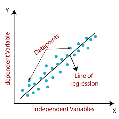
Linear Regression

2. Cost Function:
   • In linear regression, the goal is to find the best-fitting line that minimizes the error between predicted values and actual values in the training data.
   • The most commonly used cost function for linear regression is the Mean Squared Error (MSE) or the Sum of Squared Errors (SSE). It is defined as:
     

• J(b0, b1) is the cost function to be minimized.
• m is the number of data points in the training set.
• (xi, yi) represents each data point in the training set.
• b0 and b1 are the coefficients to be learned.

3. Optimization (Gradient Descent):
   • The optimization process in linear regression involves finding the values of b0 and b1 that minimize the cost function J(b0, b1).
   • Gradient Descent is a common optimization algorithm used for this purpose. It works by iteratively adjusting the values of b0 and b1 to reach the minimum of the cost function.
   • The update rules for gradient descent are as follows:
     

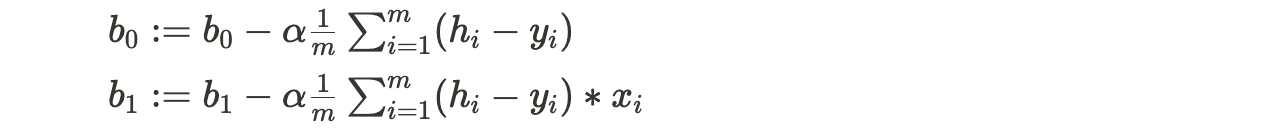
• alpha is the learning rate, which controls the step size during each iteration.
• $h_i$ is the predicted value for the i-th data point.
• The summation terms represent the partial derivatives of the cost function with respect to $b_0$ and $b_1$, respectively.
• The process continues until the algorithm converges to a minimum, where the cost function is at its lowest point, indicating the best-fit line.

Linear regression is a simple yet powerful algorithm, especially when the relationship between the independent and dependent variables is approximately linear. It's widely used for tasks like predicting stock prices, estimating product demand, and analyzing the impact of variables on an outcome.

Logistic Regression

Logistic Regression is a widely used classification algorithm in machine learning, despite its name including "regression." It is employed for binary and multiclass classification tasks, where the goal is to predict the probability of an instance belonging to a particular class. Logistic regression is particularly useful when the output is binary, meaning it falls into one of two categories (e.g., spam or not spam, yes or no, positive or negative).

Here are the key components of a logistic regression model:

1. Logistic Regression Model:
   • The logistic regression model takes a linear combination of input features and transforms it into a probability using the logistic or sigmoid function. It is represented as follows:
     

• P(Y = 1|X) is the probability that the instance belongs to class 1 given the input features X.
• x1, x2, ..., xn are the independent variables (features).
• b0, b1, b2, ..., bn are the coefficients or weights associated with each feature.
• e is the base of the natural logarithm.
• The logistic function maps the linear combination to a value between 0 and 1, which can be interpreted as the probability of the instance belonging to class 1.

2. Sigmoid Function:
   • The sigmoid function, denoted as $\sigma(z)$, is the core of logistic regression and is used to transform the linear combination of input features into a probability.
   • The sigmoid function is defined as:
     

• z represents the linear combination of input features and coefficients.
• The sigmoid function has an S-shaped curve, which ensures that the output is bounded between 0 and 1. As z becomes large and positive, \sigma(z) approaches 1, indicating a high probability of class 1. Conversely, as z becomes large and negative, \sigma(z) approaches 0, indicating a low probability of class 1.

3. Cost Function (Log Loss or Binary Cross-Entropy):
   • The cost function in logistic regression is designed to measure the error between the predicted probabilities and the true class labels.
   • For binary classification, the cost function is commonly known as the log loss or binary cross-entropy. It is defined as:
     

• J(b) is the cost function to be minimized.
• m is the number of data points in the training set.
• yi is the true class label (0 or 1) for the i-th instance.
• yi^ is the predicted probability that the i-th instance belongs to class 1.
• The cost function penalizes the model heavily if it predicts a high probability for the wrong class and rewards it when the predicted probability aligns with the true class.
• The cost function penalizes the model heavily if it predicts a high probability for the wrong class and rewards it when the predicted probability aligns with the true class.

The training of a logistic regression model typically involves minimizing the cost function, often using optimization techniques like gradient descent, to find the optimal values for the coefficients b0, b1, b2, ..., bn. Once trained, the model can make predictions for new data points by calculating the probability of belonging to the positive class and making a decision based on a predefined threshold (e.g., 0.5).

Logistic regression is widely used in various applications such as spam detection, disease diagnosis, customer churn prediction, and sentiment analysis, where binary or multiclass classification is required.

Decision Trees

Decision Trees are versatile and widely used classification algorithms in machine learning. They are also used for regression tasks (referred to as regression trees). Decision trees are particularly appealing because they can handle both categorical and numerical features and provide interpretable models, making them useful in various domains, including finance, healthcare, and marketing.

Here are the key components and concepts related to decision trees:

1. Tree Construction:
   • A decision tree consists of nodes that represent decisions or questions, branches that represent possible answers or choices, and leaves that represent class labels or regression values.
   • The process of constructing a decision tree involves recursively partitioning the dataset into subsets based on the values of the input features.
   • The goal is to split the data in a way that maximizes the homogeneity of the classes within each subset. This is typically measured using metrics like Gini impurity or information gain.
2. Information Gain:
   • Information gain is a metric used to evaluate the quality of a split in a decision tree. It quantifies the reduction in uncertainty or disorder achieved by a particular split.
   • In classification tasks, information gain is often used in conjunction with entropy (a measure of disorder) to calculate the gain. The formula for information gain is as follows:
     

• The objective is to select the split that results in the highest information gain, meaning it provides the most valuable information for classification.

3. Tree Pruning:
   • Decision trees are prone to overfitting, where they learn the training data too well, capturing noise and making them less generalizable to new data.
   • Tree pruning is a technique used to reduce the size of a decision tree by removing branches that do not significantly improve its predictive performance.
   • Pruning can be based on criteria like the minimum number of samples in a leaf node or the maximum depth of the tree.
4. Handling Categorical Features:
   • Decision trees can naturally handle categorical features. When splitting a node, they evaluate all possible values of a categorical feature to find the best split.
   • One common approach to handling categorical features is to use binary encoding or one-hot encoding to represent them as numerical values. This allows the tree to treat categorical features as if they were numerical.
5. Preventing Overfitting:
   • Decision trees are prone to overfitting, especially when they are deep and capture noise in the data. Several strategies can help prevent overfitting:
     • Limiting the maximum depth of the tree.
     • Setting a minimum number of samples required to split a node.
     • Pruning the tree as mentioned earlier.
     • Using ensemble methods like Random Forests or Gradient Boosting, which combine multiple decision trees to improve generalization.

Decision trees offer interpretability and are suitable for both binary and multiclass classification tasks. However, they can be sensitive to small changes in the data and might create complex trees if not pruned properly. Therefore, careful tuning and validation are crucial to getting the best performance from decision trees.

Other Classification Algorithms

Naive Bayes Algorithm:

The Naive Bayes algorithm is a probabilistic classification method based on Bayes' theorem, which calculates the probability of a hypothesis (class) given some observed evidence (features). Despite its simplicity, Naive Bayes often performs well in various classification tasks, especially in text classification and spam detection. Here's how it works:

1. Bayes' Theorem:

• Bayes' theorem is a fundamental concept in probability theory that relates the conditional probability of an event to the probabilities of other related events. It can be stated as:
  
• P(A|B) is the probability of event A given that event B has occurred.
• P(B|A) is the probability of event B given that event A has occurred.
• P(A) and P(B) are the probabilities of events A and B, respectively.

2. Naive Assumption:

• The "naive" part of Naive Bayes comes from an assumption that the features used for classification are conditionally independent, given the class label. In other words, features are assumed to have no relationship with each other once the class is known. This simplifying assumption is made for computational efficiency.

3. Classification:

• To classify a new data point, Naive Bayes calculates the posterior probability of each class and assigns the class with the highest posterior probability as the predicted class.
• The probability is calculated using Bayes' theorem as follows:
  
• P(Ck|X) is the posterior probability of class Ck given the features X.
• P(X|Ck) is the likelihood, which represents the probability of observing the features X given class Ck.
• P(Ck) is the prior probability of class Ck.
• P(X) is the evidence, which is the probability of observing the features X.

4. Strengths and Weaknesses:

• Strengths:
  • Simplicity and computational efficiency: Naive Bayes is fast to train and make predictions.
  • Can handle high-dimensional data: It performs well even when there are many features.
  • Suitable for text data: Naive Bayes is widely used in text classification tasks like spam detection and sentiment analysis.
• Weaknesses:
  • Naive independence assumption: The assumption that features are independent can lead to suboptimal results when this assumption is violated.
  • Lack of model interpretability: Naive Bayes doesn't provide insights into feature importance or the relationships between features.
  • Sensitive to feature distribution: It may not perform well if the data doesn't conform to the assumed probability distribution (e.g., Gaussian or multinomial for different Naive Bayes variants).

K-Nearest Neighbors (KNN):

K-Nearest Neighbors is a distance-based classification algorithm. It classifies a new data point by finding the K training examples (neighbors) that are closest to it in feature space and then taking a majority vote among these neighbors. Here's how it works:

Distance Metric:

• KNN uses a distance metric (e.g., Euclidean distance or Manhattan distance) to measure the similarity or dissimilarity between data points.

Classification:

• To classify a new data point, KNN finds the K nearest neighbors in the training data based on the chosen distance metric.
• It assigns the class label that is most frequent among these K neighbors to the new data point.

Strengths and Weaknesses:

• Strengths:
  • Simplicity: KNN is easy to understand and implement.
  • No assumptions about data distribution: It can work well with data that doesn't follow specific probability distributions.
  • Works for both classification and regression: KNN can be used for regression by taking the mean or median of the target values of the nearest neighbors.
• Weaknesses:
  • Computationally expensive: KNN needs to calculate distances to all training data points for each prediction, which can be slow for large datasets.
  • Sensitivity to K value: The choice of K can impact the model's performance. Smaller values of K may lead to noisy predictions, while larger values may smooth out decision boundaries.
  • Sensitive to feature scaling: Features with larger scales can dominate the distance calculation, so feature scaling is often necessary.
  • Can be affected by irrelevant features: The algorithm doesn't automatically select or weight features, so irrelevant features can affect its performance.

The choice between Naive Bayes and KNN (or other algorithms) depends on the specific characteristics of the dataset and the problem at hand. Naive Bayes is a probabilistic method that makes strong independence assumptions, while KNN is a distance-based method that doesn't assume any specific distribution of the data. Therefore, their performance can vary based on the data and problem complexity.

Support Vector Machines (SVM)

Support Vector Machine (SVM) is a powerful and versatile classification technique used in machine learning. It is particularly effective for both linear and nonlinear classification problems. SVM aims to find the optimal hyperplane that best separates different classes in the feature space, and it can handle both binary and multiclass classification tasks.

Here are the key concepts associated with SVM:

1. Margin:
   • In SVM, a margin is a gap between the closest data points (support vectors) of different classes and the decision boundary (hyperplane).
   • The goal of SVM is to maximize this margin while minimizing classification errors. A larger margin typically leads to better generalization to new, unseen data.
   • Support vectors are the data points that lie on or within the margin and are crucial in defining the optimal hyperplane.
2. Kernel Functions:
   • SVM can be used not only for linear classification (where a straight line separates classes) but also for nonlinear classification tasks (where classes are not separable by a straight line).
   • Kernel functions play a key role in SVM by mapping the original feature space into a higher-dimensional space where the classes become linearly separable.
   • Common kernel functions include:
     • Linear Kernel: Used for linearly separable data.
     • Polynomial Kernel: Maps data into a higher-dimensional space using polynomial functions.
     • Radial Basis Function (RBF) Kernel: Often used for nonlinear problems, it maps data into an infinite-dimensional space.
     • Sigmoid Kernel: Maps data using a sigmoid function.
3. Hyperplane Optimization:
   • The main objective of SVM is to find the optimal hyperplane that maximizes the margin while minimizing classification errors.
   • The equation of the hyperplane is typically represented as:
     w . x + b = 0

• w is the weight vector perpendicular to the hyperplane.
• x is the input feature vector.
• b is the bias term.
• SVM seeks to find w and b that maximize the margin while satisfying the constraint that data points are correctly classified. This is typically formulated as a convex optimization problem.

4. Strengths and Weaknesses:
   • Strengths:
     • Effective for high-dimensional data: SVM can handle datasets with many features.
     • Versatile: It can be used for both linear and nonlinear classification tasks using appropriate kernel functions.
     • Robust to outliers: SVM is less sensitive to outliers compared to some other classifiers.
     • Theoretical foundation: SVM has a strong theoretical foundation in convex optimization and margin maximization.
   • Weaknesses:
     • Computational complexity: Training an SVM can be computationally expensive, especially for large datasets.
     • Tuning hyperparameters: Selecting the right kernel and tuning hyperparameters can be challenging.
     • Lack of probabilistic outputs: SVM does not provide probability estimates for class membership directly, although this can be estimated using techniques like Platt scaling.

SVM is a versatile and powerful classifier, and its performance depends on careful selection of kernel functions and tuning of hyperparameters. It is well-suited for a wide range of applications, including text classification, image classification, and bioinformatics, where the data may not be linearly separable in the original feature space.

Model Evaluation Metrics

Evaluation metrics are used to assess the performance of machine learning models in both regression and classification tasks. The choice of the appropriate metric depends on the nature of the problem and the goals of the analysis. Here are some common evaluation metrics for regression and classification tasks:

Regression Metrics:

1. Mean Squared Error (MSE):
   • Measures the average squared difference between the predicted values and the actual values.
   • It gives more weight to large errors, making it sensitive to outliers.
   • MSE is suitable when you want to penalize large prediction errors.
2. Root Mean Squared Error (RMSE):
   • RMSE is the square root of the MSE.
   • It is in the same units as the target variable, making it more interpretable.
   • Like MSE, RMSE is suitable for tasks where you want to penalize large errors.
3. Mean Absolute Error (MAE):
   • Measures the average absolute difference between the predicted values and the actual values.
   • It is less sensitive to outliers compared to MSE.
   • MAE is useful when you want to understand the magnitude of errors in the predictions.
4. R-squared (R²) or Coefficient of Determination:
   • Measures the proportion of the variance in the target variable that is predictable from the independent variables.
   • R² values range from 0 to 1, with higher values indicating a better fit.
   • R² is useful when you want to assess the goodness of fit of the model.

Classification Metrics:

1. Accuracy:
   • Measures the proportion of correctly predicted instances out of all instances.
   • It is suitable when the classes are balanced, and false positives and false negatives have similar consequences.
2. Precision:
   • Precision measures the proportion of true positive predictions out of all positive predictions.
   • It is useful when the cost of false positives is high, and you want to minimize the number of false alarms.
3. Recall (Sensitivity or True Positive Rate):
   • Measures the proportion of true positive predictions out of all actual positive instances.
   • It is important when the cost of false negatives is high, and you want to capture as many positive cases as possible.
4. F1-Score:
   • F1-Score is the harmonic mean of precision and recall.
   • It balances precision and recall and is suitable when you want to find a compromise between false positives and false negatives.
5. ROC Curve (Receiver Operating Characteristic) and AUC (Area Under the ROC Curve):
   • ROC curves plot the true positive rate (recall) against the false positive rate at various thresholds.
   • AUC quantifies the overall performance of a classification model, regardless of the threshold.
   • ROC and AUC are suitable when you want to evaluate a model's performance across different trade-offs between true positives and false positives.

When to Use Specific Metrics:

• Regression Metrics:
  • MSE and RMSE are commonly used when you want to minimize the impact of large errors, such as in financial modeling or engineering applications.
  • MAE is appropriate when you want a more interpretable metric that considers the absolute magnitude of errors.
  • R² is useful when you want to assess how well the model explains the variance in the target variable.
• Classification Metrics:
  • Accuracy is suitable when the classes are balanced and you want to measure overall correctness.
  • Precision is important when you want to minimize false positives, like in medical diagnosis or fraud detection.
  • Recall is crucial when you want to capture as many positive cases as possible, such as in disease screening or anomaly detection.
  • F1-Score is a good choice when you need a balance between precision and recall.
  • ROC and AUC are helpful when you want to evaluate the model's performance across different decision thresholds and when class imbalance is present.

The choice of metric should align with the specific goals and requirements of the problem and should consider the real-world consequences of false positives and false negatives.

Cross-Validation

Cross-validation is a critical technique in machine learning used to assess the performance and generalization ability of a predictive model. It involves partitioning the dataset into subsets for training and testing, allowing the model to be evaluated on different subsets of the data. Cross-validation provides a more robust estimate of a model's performance compared to a single train-test split.

Importance of Cross-Validation:

1. Robust Performance Estimation: Cross-validation provides a more accurate estimate of a model's performance by testing it on multiple subsets of the data. This helps to reduce the risk of obtaining overly optimistic or pessimistic performance estimates.
2. Avoiding Overfitting: It helps in detecting overfitting, where a model performs well on the training data but poorly on unseen data. Cross-validation allows you to assess how well a model generalizes to new data.
3. Hyperparameter Tuning: Cross-validation is used in hyperparameter tuning (e.g., selecting the best values for parameters like learning rates, tree depths, or regularization strengths). It helps in finding hyperparameters that result in the best model performance on unseen data.
4. Data Utilization: Cross-validation ensures that all data points are used for both training and testing, maximizing the use of available information.

There are several methods of cross-validation, with most common approach being k-fold cross-validation:

1. K-Fold Cross-Validation:
   • In k-fold cross-validation, the dataset is divided into k approximately equal-sized subsets (or folds).
   • The model is trained and evaluated k times, each time using a different fold as the test set and the remaining k-1 folds as the training set.
   • The final performance metric is usually the average of the k evaluation results.
   • Common values for k include 5 and 10, but the choice can depend on the dataset size and computational resources.

• K-fold cross-validation provides a balance between the computational cost (more efficient than leave-one-out) and reliable performance estimation (less prone to variability compared to a single train-test split).

Model Evaluation and Hyperparameter Tuning

Hyperparameters play a crucial role in machine learning models, and their proper tuning is essential for achieving good model performance. Hyperparameters are parameters that are not learned from the data but are set before training the model. They control aspects of the model's behavior, architecture, and complexity. Here's why hyperparameters are important:

1. Model Performance: Hyperparameters significantly impact a model's performance. Suboptimal hyperparameter choices can lead to models that underfit (too simple) or overfit (too complex) the data, resulting in poor generalization to unseen data.
2. Generalization: Proper hyperparameter tuning helps ensure that a model generalizes well to new, unseen data. It helps find the right balance between fitting the training data and avoiding overfitting.
3. Computational Efficiency: Efficiently chosen hyperparameters can lead to faster model training and inference. For example, selecting an appropriate learning rate or regularization strength can speed up convergence.
4. Interpretability: Hyperparameters can influence the interpretability of a model. For example, the depth of a decision tree or the number of hidden layers in a neural network can affect the model's interpretability.

To find the best hyperparameters for a machine learning model, you can use techniques like Grid Search and Random Search:

Grid Search:

• Grid search is a systematic approach to hyperparameter tuning.
• It involves specifying a set of hyperparameters and their possible values in advance.
• The technique then exhaustively evaluates all possible combinations of hyperparameters by training and testing the model on each combination.
• Grid search is a brute-force method, as it evaluates every combination, making it more suitable for smaller hyperparameter search spaces.
• It guarantees that you'll explore all combinations within the specified search space.
• It provides a clear and systematic way to tune hyperparameters.
• It can be computationally expensive, especially when the search space is large.
• It may not be efficient when some hyperparameters are less influential than others, as it allocates equal effort to all hyperparameters.

Random Search:

• Random search is a more efficient alternative to grid search.
• Instead of evaluating all combinations of hyperparameters, it randomly samples a subset of combinations.
• The random search process can be guided by specifying a probability distribution for each hyperparameter.
• Random search is often preferred when the search space is large or when certain hyperparameters are believed to have a more significant impact on model performance.
• It is computationally more efficient than grid search, especially for large search spaces.
• It is more likely to explore promising hyperparameter combinations due to the random sampling.
• It may not guarantee that all combinations within the search space are explored.
• There's no guarantee of finding the absolute best hyperparameters, as the search process is stochastic.

The choice between grid search and random search depends on factors like the available computational resources, the size of the hyperparameter search space, and the specific requirements of the problem. In practice, random search is often favored due to its efficiency and its ability to discover good hyperparameter combinations within a reasonable amount of time.

Conclusion

In the realm of machine learning, understanding key concepts and techniques is essential for building effective models and making informed decisions. From supervised learning algorithms like linear regression and logistic regression to more advanced methods like decision trees, SVMs, and Naive Bayes, the toolbox of machine learning is vast and diverse. Moreover, the significance of proper evaluation, cross-validation, and hyperparameter tuning cannot be overstated in ensuring models generalize well to new data and perform optimally. Armed with these fundamentals, you'll be better equipped to approach a wide range of machine learning problems.

Key Takeaways:

• Supervised learning involves training models using labeled data, making it suitable for both regression and classification tasks.
• Linear regression predicts continuous values, while logistic regression classifies data into categories using a sigmoid function.
• Decision trees are versatile classifiers that use tree structures for decision-making and can handle both categorical and numerical features.
• Naive Bayes is a probabilistic classification algorithm based on Bayes' theorem, with an assumption of feature independence.
• Evaluation metrics differ for regression (MSE, RMSE, MAE) and classification (Accuracy, Precision, Recall, F1-Score), chosen based on problem specifics.
• Cross-validation (k-fold) is crucial for robust model assessment and hyperparameter tuning.
• Hyperparameters control model behavior and must be carefully tuned using techniques like Grid Search or Random Search.

Practice Questions

1: What is the primary goal of feature engineering in supervised machine learning?

A. To reduce model complexity 

B. To improve model interpretability 

C. To enhance model performance 

D. To increase the number of training samples

Answer

C. To enhance model performance

Explanation: Feature engineering aims to create new features or transform existing ones to provide the machine learning model with more relevant information, ultimately improving its predictive performance.

2. Which of the following is NOT a classification metric for evaluating supervised machine learning models?

A. Mean Absolute Error (MAE) 

B. F1-Score 

C. Area Under the ROC Curve (AUC-ROC) 

D. Precision

Answer

A. Mean Absolute Error (MAE)

Explanation: MAE is a regression metric, not a classification metric. It measures the average absolute difference between predicted and actual values in regression tasks.

3. In a binary classification problem, you have a highly imbalanced dataset with 95% of the samples in Class A and 5% in Class B. Which evaluation metric is most suitable for assessing model performance in this scenario?

A. Accuracy 

B. Precision 

C. Recall 

D. F1-Score

Answer

B. Precision

Explanation: In highly imbalanced datasets, accuracy can be misleading. Precision, which focuses on the true positives among the predicted positives, is more suitable as it accounts for false positives in such scenarios.

4. When training a support vector machine (SVM) classifier, what is the purpose of the regularization parameter C?

A. To control the margin width 

B. To control the kernel function 

C. To control overfitting 

D. To control the number of support vectors

Answer

C. To control overfitting

Explanation: The regularization parameter C in an SVM controls the trade-off between maximizing the margin and minimizing the classification error. A smaller C encourages a larger margin but may lead to underfitting, while a larger C allows for a smaller margin but may lead to overfitting. This answer is correct.

5. In a decision tree, which attribute selection measure assesses the impurity reduction achieved by splitting the data on a particular attribute?

A. Gini Index 

B. Information Gain 

C. Chi-Square 

D. Entropy

Answer

Answer: B. Information Gain

Explanation: Information Gain is the attribute selection measure in a decision tree that assesses the impurity reduction achieved by splitting the data on a particular attribute. It quantifies how much information is gained about the class variable (target) by knowing the value of the attribute. The attribute with the highest Information Gain is chosen as the splitting attribute because it maximizes the reduction in uncertainty about the class labels after the split.

• Gini Index and Entropy are also commonly used impurity measures in decision trees. They assess the impurity or disorder of a dataset, and the attribute that reduces impurity the most is selected.
• Chi-Square is typically used for feature selection in the context of categorical data and is not a primary attribute selection measure for decision trees.